- 製造業出身のデータサイエンティストがお送りする記事
- 今回は製造業で使える異常検知手法を実装し整理しました。
はじめに
前回の異常検知手法(MSPC)に引続き、今回は疎構造学習による異常検知手法を整理しました。
疎構造学習による異常検知とは
異常検知手法として有名なホテリングの$T^2$法や$MSPC$は平均値が変化しないデータの監視をする時に用いる手法です。
一方、製造現場では必ずしもそのようなデータばかりではなく、変数間に一定の関係性を保ちながら値が変化するデータ構造の設備や操業データがあるかと思います。その時に変数間の関係(相関関係、等)に着目した異常検知手法の一つに疎構造学習による異常検知手法があります。
手法の概要
- 変数間の相関関係を求めるために、データの背後に多変量正規分布を仮定し、精度行列(共分散行列の逆数)を求めます。
- 実データでは意味のある相関関係のみを抽出することが困難(ノイズの影響)なため、今回は、正則化項付きの共分散行列推定(Sparse Inverse Covariance Matrix Estimation)を用います。
- 異常度は正常時と評価時(オンライン監視時)の確率分布の差(KL距離)を異常度として定義します。
手法の詳細は(異常検知と変化点検知)を読んで頂けると理解が深まるかと思います。私もこの本を読んで勉強し、実際の業務で実践しました。
疎構造学習による異常検知手法の実装
今回、サンプル用にUCI機械学習リポジトリのWater Treatment Plantというデータセットを使用しました。
正常データを100件、残りの279件を評価データとして正常状態からどれだけ逸脱しているのかを見ました。
pythonのコードは下記の通りです。
# 必要なライブラリーのインポート
import pandas as pd
import numpy as np

from matplotlib import pyplot as plt
%matplotlib inline
from scipy import stats

from sklearn.preprocessing import StandardScaler
from sklearn.neighbors.kde import KernelDensity
from sklearn.covariance import GraphicalLassoCV

df = pd.read_csv('watertreatment_mod.csv', encoding='shift_jis', header=0, index_col=0)
TimeIndices = df.index
df.head()

window_size = 10
cr = 0.99
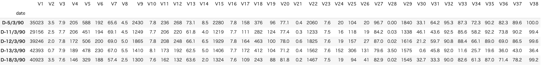
インプットデータは上記のような感じです。
次に学習データと評価データを分割し、標準化を行っていきます。
# 分割ポイント
split_point = 100
# 学習データ(train)と評価データ(test)に分割
train_df = df.iloc[:(split_point-1),]
test_df = df.iloc[split_point:,]

# データを標準化
sc = StandardScaler()
sc.fit(train_df)
train_df_std = sc.transform(test_df)
test_df_std = sc.transform(test_df)
次に共分散の推定を行います。
# 共分散の推定
n_samples, n_features = train_df_std.shape
emp_cov = np.dot(train_df_std.T, train_df_std) / n_samples

model = GraphicalLassoCV()
model.fit(train_df_std)
cov_ = model.covariance_
prec_ = model.precision_
次にKL距離を求める関数を定義しておきます。
def Calc_KL(cov_, prec_, xtest):
    """KL距離の計算を行う

    Parameters
    ----------
    cov_ (np.array)     : 学習データの共分散行列
    prec_ (np.array)    : 学習データの精度行列
    df (pd.DataFrame)   : データセット

    Returns
    -------
    d_ab (pd.DataFrame) : KL距離

    """
    n_samples, n_features = xtest.shape

    d_abp=np.zeros(n_features)
    d_abm=np.zeros(n_features)
    d_ab=np.zeros(n_features)

    model_test = GraphicalLassoCV()
    try:
        model_test.fit(xtest)
    except FloatingPointError:
        print("floating error")
        return d_ab

    cov__test = model_test.covariance_
    prec__test = model_test.precision_

    # 変数毎に相関の崩れの大きさを計算する
    for i in range(n_features):
        temp_prec_a = np.r_[prec_[i:n_features,:], prec_[0:i,:]]
        temp_prec_a = np.c_[temp_prec_a[:,i:n_features], temp_prec_a[:,0:i]]
        temp_prec_b = np.r_[prec__test[i:n_features,:], prec__test[0:i,:]]
        temp_prec_b = np.c_[temp_prec_b[:,i:n_features], temp_prec_b[:,0:i]]
        temp_cov_a = np.r_[cov_[i:n_features,:], cov_[0:i,:]]
        temp_cov_a = np.c_[temp_cov_a[:,i:n_features], temp_cov_a[:,0:i]]
        temp_cov_b = np.r_[cov__test[i:n_features,:], cov__test[0:i,:]]
        temp_cov_b = np.c_[temp_cov_b[:,i:n_features], temp_cov_b[:,0:i]]
        La = temp_prec_a[:-1, :-1]
        la = temp_prec_a[:-1, -1]
        lama = temp_prec_a[-1, -1]
        Wa = temp_cov_a[:-1, :-1]
        wa = temp_cov_a[:-1, -1]
        sigmaa = temp_cov_a[-1, -1]
        Lb = temp_prec_b[:-1, :-1]
        lb = temp_prec_b[:-1, -1]
        lamb = temp_prec_b[-1, -1]
        Wb = temp_cov_b[:-1, :-1]
        wb = temp_cov_b[:-1, -1]
        sigmab = temp_cov_b[-1, -1]

        d_abp[i] = np.dot(wa, la)+0.5*(np.dot(np.dot(lb, Wb), lb)-np.dot(np.dot(la, Wa), la))+0.5*(np.log(lama/lamb)+sigmaa-sigmab)
        d_abm[i] = np.dot(wb, lb)+0.5*(np.dot(np.dot(la, Wa), la)-np.dot(np.dot(lb, Wb), lb))+0.5*(np.log(lamb/lama)+sigmab-sigmaa)
        d_ab[i] = max(-d_abp[i], -d_abm[i])

    return d_ab
次に管理限界をカーネル密度推定によって算出する関数を用意します。
def cl_limit(x, cr=0.99):
    """管理限界の計算を行う

    Parameters
    ----------
    x (np.array) : KL距離
    cr (float)   : 管理限界の境界

    Returns
    -------
    cl (float)   : 管理限界の境界点

    """
    X = x.reshape(np.shape(x)[0],1)
    bw= (np.max(X)-np.min(X))/100
    kde = KernelDensity(kernel='gaussian', bandwidth=bw).fit(X)
    X_plot = np.linspace(np.min(X), np.max(X), 1000)[:, np.newaxis]
    log_dens = kde.score_samples(X_plot)
    prob = np.exp(log_dens) / np.sum(np.exp(log_dens))
    calprob = np.zeros(np.shape(prob)[0])
    calprob[0] = prob[0]
    for i in range(1,np.shape(prob)[0]):
        calprob[i]=calprob[i-1]+prob[i]

    cl = X_plot[np.min(np.where(calprob>cr))]

    return cl
学習データをクロスバリデーションをして管理限界を算出します。
K = 5
cv_data_size = np.int(np.shape(train_df_std)[0]/5)
n_train_samples = np.shape(train_df_std)[0]
counter = 0

for i in range(K):

    cv_train_data=np.r_[train_df_std[0:i*cv_data_size,], train_df_std[(i+1)*cv_data_size:,]]
    if i < K-1:
        cv_test_data=train_df_std[i*cv_data_size:(i+1)*cv_data_size,]
    else:
        cv_test_data=train_df_std[i*cv_data_size:,]

    model_cv = GraphicalLassoCV()
    model_cv.fit(cv_train_data)
    cov__cv = model.covariance_
    prec__cv = model.precision_

    for n in range(window_size, np.shape(cv_test_data)[0]):
        count = i*cv_data_size + n
        tempX = cv_test_data[n-window_size:n,:]
        d_ab_temp = Calc_KL(cov__cv, prec__cv, tempX)

        if 0 == counter:
            d_ab = d_ab_temp.reshape(1,n_features)
            TimeIndices2 = TimeIndices[count]
        else:
            d_ab = np.r_[d_ab,d_ab_temp.reshape(1,n_features)]
            #ここでerror
            TimeIndices2 = np.vstack((TimeIndices2,TimeIndices[count]))

        counter = counter + 1

split_point = np.shape(d_ab)[0]
d_ab_cv = d_ab[np.sum(d_ab,axis=1)!=0,:]

cl = np.zeros([n_features])
for i in range(n_features):
    cl[i] = cl_limit(d_ab_cv[:,i],cr)
最後に評価データの共分散を推定し、可視化します。
# 評価データに対しても共分散を推定
n_test_samples = np.shape(test_df_std)[0]

for n in range(window_size, n_test_samples):
    tempX = test_df_std[n-window_size:n,:]

    d_ab_temp = Calc_KL(cov_, prec_, tempX)

    d_ab = np.r_[d_ab,d_ab_temp.reshape(1,n_features)]
    TimeIndices2 = np.vstack((TimeIndices2,TimeIndices[n+n_train_samples]))

x2 = [0, np.shape(d_ab)[0]]
x3 = [split_point, split_point]
x = range(0, np.shape(TimeIndices2)[0],20)
NewTimeIndices = np.array(TimeIndices2[x])
for i in range(38):
    plt.figure(figsize=(200, 3))
    plt.subplot(1, 38, i+1)
    plt.title('%s Contribution' % (i))
    plt.plot(d_ab[:, i], marker="o")
    plt.xlabel("Time")
    plt.ylabel("Contribution")
    plt.xticks(x,NewTimeIndices,rotation='vertical')
    y2 = [cl[i],cl[i]]
    plt.plot(x2,y2,ls="-", color = "r")
    y3 = [0, np.nanmax(d_ab[:,i])]
    plt.plot(x3,y3,ls="--", color = "b")

plt.show()
さいごに
最後まで読んで頂き、ありがとうございました。
今回は、疎構造学習による異常検知について実装しました。
訂正要望がありましたら、ご連絡頂けますと幸いです。
参考文献
- 井出剛・杉山将 『異常検知と変化検知』, 2015年, 講談社