今回の目的
今回は皆さんが、高校物理、大学電磁気学で学習するアンペールの法則を用いた磁界の様子をPythonとMatplotlibを用いて可視化したいと思います。使用する式自体はとてもシンプルな公式のみを使うことになりますので電磁気を怖がらずに見てください。
プログラムを切り取って解説していますが、全体をまとめたものは一番最後のプログラム全体にあるので、そちらをコピペして遊んでみてから読んでもいいかもしれないです!
出力結果
先に出力結果を示します。左が磁界の強さを高低差で表した図で、右が円柱回りの磁界の大きさと方向を色と矢印で表した結果になります。
少し工夫をしてマウスでなぞると片方の円柱を動かせるようにもしました。

流れ
今回の記事では以下のような流れで進みます。
-
アンペールの法則の紹介 - アンペールの法則を用いた磁界を導出する式を求める
- 磁界を求める式をプログラムに落とし込む
-
matplotlibにて可視化
磁界を求めるための式の導出
アンペールの法則
アンペールの法則は、式で以下のように表されます。
\oint_C H\cdot ds = I
意味は、
閉じた経路に沿って磁場の大きさを足し合わせると、閉じた経路を貫く電流の大きさと等しい [参照:Wikipedia]
というものです。この式を用いることで直線電流の周りに発生する磁界を求めることが簡単にできます。
円柱導体に電流を流した時の円柱内外の磁界を求める
半径 $r_o$ の円柱に電流 $I$を流すとアンペールの法則により、その周りに磁界が発生します。
磁界は向きと大きさを持つベクトルで、右ねじの法則の方向に円柱周りに発生します。以下のように真ん中に円柱があり、奥から手前に向けて電流が流れているときには反時計回りに磁界が発生します。黒い円が円柱の外枠を表しており、色が赤いほど強い磁界が発生しています。

ここから式を導出しますが、円柱内外で場合分けをする必要があります。円柱内では測定する磁界の位置によって、その内側を流れる電流の総和が変わってくるからです。
1. 円柱外
電流は、ある任意の半径 $r$ の円周上の磁界を周回積分した値となるので、次回の大きさを $H_{out}$とし、
2\pi rH_{out} = I
となり、円柱外の磁界の大きさは以下のようになります。
H_{out} = \frac{I}{2\pi r}
2. 円柱内
円柱内の電流の大きさは磁界を求める位置 $r$によって変わり、以下のようになります。
2\pi rH_{in} = I\frac{\pi r^2}{\pi r_o^2}
これより、円柱内の大きさは以下のようになります。
H_{in} = \frac{rI}{2\pi r_o^2}
これで使用する数式の準備は完了です。ではプログラムを作成してきましょう。
フローチャート
実行にあたってまずプログラムの大まかな流れをフローチャートで説明します。

プログラム
ライブラリのインポート
-
numpyは行列などの計算用 -
matplotlibからは、円、カラーマップのライブラリもインポートします。
import numpy as np
import numpy.matlib
import matplotlib.pyplot as plt
import matplotlib.patches as patches
from matplotlib import cm
初期値と変数の定義
#set initial value
Nd=26 # number of data (arrows for each axis)
x_len=200 # figure size
y_len=200 # figure size

#first cylinder info
r_0=50 # radius
x_0,y_0=-100,0 # position of the center
current_0=100 # current value
a=Cal(r_0,x_0,y_0,Nd,x_len,y_len,current_0)
U_0,V_0=a.Hinout()

#set second cylinder info as initial value
r_1_0=50 # radius
x_1,y_1=0,0 # position of the center
current_1=100 # current value
b=Cal(r_1_0,x_1,y_1,Nd,x_len,y_len,current_1)
U_1,V_1=b.Hinout()
計算を行う
初期設定・座標軸作成
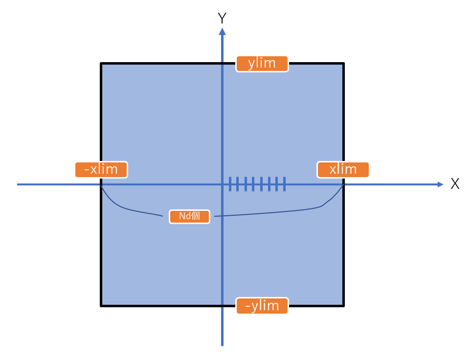
円の半径、中心座標、図の$x$,$y$座標の上限下限値、計算データ数を決定し、numpy配列を利用して、$x$座標、$y$座標を「データ数$\times$データ数」の行列にします。
下の図のように、xlimとylimで座標の最大最小値を決定し、Nd個に分けてnp.linspaceとnp.matlib.repmatを利用して2次元の配列を作成します。
    def __init__(self,r_0,x_center,y_center,Nd,x_len,y_len,current):
        self.r_0=r_0 # radius of the circle
        self.x_center=x_center # x-coordinate of the circle center
        self.y_center=y_center # y-coordinate of the circle center
        self.cur=current # current value flowing through the cylinder
        # set x and y limit of figure
        self.x_min=-x_len
        self.x_max=x_len
        self.y_min=-y_len
        self.y_max=y_len
        self.Nd=Nd # number of data
        # creating x and y coordinate according number of data as ndarray
        self.x=np.linspace(self.x_min,self.x_max,self.Nd)
        self.Xmat=np.matlib.repmat(self.x,self.Nd,1)
        self.Xmat=self.Xmat.T # x-coordinate should be transposed
        self.y=np.linspace(self.y_min,self.y_max,self.Nd)
        self.Ymat=np.matlib.repmat(self.y,self.Nd,1)
メインの計算
ここで円柱それぞれによって生じる磁界の大きさをプロットされた各座標について計算して配列に格納します。フローチャートの中ではこれでループ処理が完了する部分になります。
また、後ほど磁界 $H$ を $x$ 方向 $y$ 方向に分解して、 $U$ と $V$ も同時に求めます。

    #calculation of H for outside and inside of cylinder
    def Hinout(self):
        self.H=np.zeros((Nd,Nd)) #prepare data list of H for each plot
        self.U=np.zeros((Nd,Nd))
        self.V=np.zeros((Nd,Nd))
        for i in range(0,Nd):
            for j in range(0,Nd):
                self.Xrel=self.Xmat[i][j]-self.x_center # x-coordinate relative to the center of the circle
                self.Yrel=self.Ymat[i][j]-self.y_center # y-coordinate relative to the center of the circle
                self.r=np.sqrt(self.Xrel**2+self.Yrel**2) # radius relative to the center of the circle
                if self.r < self.r_0: # when plot is inside of  the cylinder
                    self.H[i][j]=self.r*self.cur/(2*np.pi*(self.r_0**2))
                else: # when plot is outside of the cylinder
                    self.H[i][j]=self.cur/(2*np.pi*self.r)
                self.U[i][j]=-self.H[i][j]*self.Yrel/self.r # x-vector of H
                self.V[i][j]=self.H[i][j]*self.Xrel/self.r # y-vector of H
        return self.U,self.V
- 円柱内外で磁界を求める式が変わるので場合分け
- 磁界 $H$ を $U$ と $V$ に分解しておく
合成された磁界を求める
現在、2つの円柱による磁界がそれぞれ求まった状態なので、この2つの磁界をベクトルとして足し合わせることで、実際の磁界の状態を求めます。

class Add:
    def __init__(self,U_0,V_0,U_1,V_1):
        self.U_0=U_0
        self.V_0=V_0
        self.U_1=U_1
        self.V_1=V_1

    # add x and y vector of 1st and 2nd H
    def add(self):
        self.U=self.U_0+self.U_1
        self.V=self.V_0+self.V_1
        self.H=np.sqrt(self.U**2+self.V**2) # calculate the norm of H from U and V
        return self.U,self.V,self.H
これで計算が全て終わり、プロットするのに必要なデータがそろいました。ここからプロットを行います。
描画・プロット (基本)
# figure setting
fig=plt.figure()
ax1 = fig.add_subplot(1,2,2)
ax2 = fig.add_subplot(1,2,1,projection="3d")
ax1.set_box_aspect(1)

#ax1 plot 2D figure of initial H on right side
c0=patches.Circle(xy=(x_0,y_0),radius=r_0,fc="None",ec="black") # draw a circle of 1st cylinder
c1=patches.Circle(xy=(x_1,y_1),radius=r_1_0,fc="None",ec="black") # draw a circle of 2nd cylinder
ax1.add_patch(c0)
ax1.add_patch(c1)
sc=ax1.quiver(b.Xmat,b.Ymat,U,V,H,cmap=cm.rainbow) # draw a arrow related to direction of H with color
sc=ax1.scatter(a.Xmat,a.Ymat,c=H,cmap=cm.rainbow,s=2) # plot the color of H

#ax2 plot 3D surface of initial H on left side
ax2.plot_surface(a.Xmat,a.Ymat,H,cmap=cm.cool)
ax2.set_xlabel("position x")
ax2.set_ylabel("position y")
ax2.set_zlabel("H")

plt.colorbar(sc) # colorbar

plt.show()
描画・プロット ~マウスイベントを追加~
参考:matplotlibでインタラクティブにプロットしたいんじゃ
先ほどは、初期値をもとにプロットされますが、以下のようにすることでマウスを動かし、座標を逐次入力し直して新しい図を更新することが可能になります。
マウスイベントが起こった時の動作のフローチャートです。

# figure setting
fig=plt.figure()
ax1 = fig.add_subplot(1,2,2)
ax2 = fig.add_subplot(1,2,1,projection="3d")
ax1.set_box_aspect(1)

# mouse event when you hover on the figure on the right side (ax1)
def mouse_move(event):
    #clear previous image
    ax1.clear()
    ax2.clear()

    x_1,y_1=event.xdata,event.ydata # x and y data of mouse

    #calculation
    b=Cal(r_1_0,x_1,y_1,Nd,x_len,y_len,current_1) # calculate for the new position of 2nd cylinder
    U_1,V_1=b.Hinout()
    c=Add(U_0,V_0,U_1,V_1) # add U and V of 1st and 2nd cylinder
    U,V,H=c.add()

    #ax1 plot 2D figure of H on right side
    ax1.quiver(b.Xmat,b.Ymat,U,V,H,cmap=cm.rainbow)
    ax1.scatter(a.Xmat,a.Ymat,c=H,cmap=cm.rainbow,s=2)
    c0=patches.Circle(xy=(x_0,y_0),radius=r_0,fc="None",ec="black")
    c1=patches.Circle(xy=(x_1,y_1),radius=r_1_0,fc="None",ec="black")
    ax1.add_patch(c0)
    ax1.add_patch(c1)

    #ax2 plot 3D surface of H on left side
    ax2.plot_surface(a.Xmat,a.Ymat,H,cmap=cm.cool)
    ax2.set_xlabel("position x")
    ax2.set_ylabel("position y")
    ax2.set_zlabel("H")
    fig.canvas.draw_idle()

#ax1 plot 2D figure of initial H on right side
c0=patches.Circle(xy=(x_0,y_0),radius=r_0,fc="None",ec="black") # draw a circle of 1st cylinder
c1=patches.Circle(xy=(x_1,y_1),radius=r_1_0,fc="None",ec="black") # draw a circle of 2nd cylinder
ax1.add_patch(c0)
ax1.add_patch(c1)
sc=ax1.quiver(b.Xmat,b.Ymat,U,V,H,cmap=cm.rainbow) # draw a arrow related to direction of H with color
sc=ax1.scatter(a.Xmat,a.Ymat,c=H,cmap=cm.rainbow,s=2) # plot the color of H

#ax2 plot 3D surface of initial H on left side
ax2.plot_surface(a.Xmat,a.Ymat,H,cmap=cm.cool)
ax2.set_xlabel("position x")
ax2.set_ylabel("position y")
ax2.set_zlabel("H")

plt.colorbar(sc) # colorbar
plt.connect('motion_notify_event', mouse_move) # mouse event

plt.show()
プログラム全体
最後に、まとめた実行できるプログラムを紹介します。
ぜひ遊んでみてください!
import numpy as np
import numpy.matlib
import matplotlib.pyplot as plt
import matplotlib.patches as patches
from matplotlib import cm

class Cal:
    #set initial conditions
    def __init__(self,r_0,x_center,y_center,Nd,x_len,y_len,current):
        self.r_0=r_0 # radius of the circle
        self.x_center=x_center # x-coordinate of the circle center
        self.y_center=y_center # y-coordinate of the circle center
        self.cur=current # current value flowing through the cylinder
        # set x and y limit of figure
        self.x_min=-x_len
        self.x_max=x_len
        self.y_min=-y_len
        self.y_max=y_len
        self.Nd=Nd # number of data
        # creating x and y coordinate according number of data as ndarray
        self.x=np.linspace(self.x_min,self.x_max,self.Nd)
        self.Xmat=np.matlib.repmat(self.x,self.Nd,1)
        self.Xmat=self.Xmat.T # x-coordinate should be transposed
        self.y=np.linspace(self.y_min,self.y_max,self.Nd)
        self.Ymat=np.matlib.repmat(self.y,self.Nd,1)

    #calculation of H for outside and inside of cylinder
    def Hinout(self):
        self.H=np.zeros((Nd,Nd)) #prepare data list of H for each plot
        self.U=np.zeros((Nd,Nd))
        self.V=np.zeros((Nd,Nd))
        for i in range(0,Nd):
            for j in range(0,Nd):
                self.Xrel=self.Xmat[i][j]-self.x_center # x-coordinate relative to the center of the circle
                self.Yrel=self.Ymat[i][j]-self.y_center # y-coordinate relative to the center of the circle
                self.r=np.sqrt(self.Xrel**2+self.Yrel**2) # radius relative to the center of the circle
                if self.r < self.r_0: # when plot is inside of  the cylinder
                    self.H[i][j]=self.r*self.cur/(2*np.pi*(self.r_0**2))
                else: # when plot is outside of the cylinder
                    self.H[i][j]=self.cur/(2*np.pi*self.r)
                self.U[i][j]=-self.H[i][j]*self.Yrel/self.r # x-vector of H
                self.V[i][j]=self.H[i][j]*self.Xrel/self.r # y-vector of H
        return self.U,self.V

class Add:
    def __init__(self,U_0,V_0,U_1,V_1):
        self.U_0=U_0
        self.V_0=V_0
        self.U_1=U_1
        self.V_1=V_1

    # add x and y vector of 1st and 2nd H
    def add(self):
        self.U=self.U_0+self.U_1
        self.V=self.V_0+self.V_1
        self.H=np.sqrt(self.U**2+self.V**2) # calculate the norm of H from U and V
        return self.U,self.V,self.H


#set initial value
Nd=20 # number of data (arrows for each axis)
x_len=200 # figure size
y_len=200 # figure size

#first cylinder info
r_0=50 # radius
x_0,y_0=-100,0 # position of the center
current_0=100 # current value
a=Cal(r_0,x_0,y_0,Nd,x_len,y_len,current_0)
U_0,V_0=a.Hinout()

#set second cylinder info as initial value
r_1_0=50 # radius
x_1,y_1=0,0 # position of the center
current_1=100 # current value
b=Cal(r_1_0,x_1,y_1,Nd,x_len,y_len,current_1)
U_1,V_1=b.Hinout()

#add U,V by cylinder_0 and cylinder_1
c=Add(U_0,V_0,U_1,V_1)
U,V,H=c.add()

# figure setting
fig=plt.figure()
ax1 = fig.add_subplot(1,2,2)
ax2 = fig.add_subplot(1,2,1,projection="3d")
ax1.set_box_aspect(1)

# mouse event when you hover on the figure on the right side (ax1)
def mouse_move(event):
    #clear previous image
    ax1.clear()
    ax2.clear()

    x_1,y_1=event.xdata,event.ydata # x and y data of mouse

    #calculation
    b=Cal(r_1_0,x_1,y_1,Nd,x_len,y_len,current_1) # calculate for the new position of 2nd cylinder
    U_1,V_1=b.Hinout()
    c=Add(U_0,V_0,U_1,V_1) # add U and V of 1st and 2nd cylinder
    U,V,H=c.add()

    #ax1 plot 2D figure of H on right side
    ax1.quiver(b.Xmat,b.Ymat,U,V,H,cmap=cm.rainbow)
    ax1.scatter(a.Xmat,a.Ymat,c=H,cmap=cm.rainbow,s=2)
    c0=patches.Circle(xy=(x_0,y_0),radius=r_0,fc="None",ec="black")
    c1=patches.Circle(xy=(x_1,y_1),radius=r_1_0,fc="None",ec="black")
    ax1.add_patch(c0)
    ax1.add_patch(c1)

    #ax2 plot 3D surface of H on left side
    ax2.plot_surface(a.Xmat,a.Ymat,H,cmap=cm.cool)
    ax2.set_xlabel("position x")
    ax2.set_ylabel("position y")
    ax2.set_zlabel("H")

    fig.canvas.draw_idle()

#ax1 plot 2D figure of initial H on right side
c0=patches.Circle(xy=(x_0,y_0),radius=r_0,fc="None",ec="black") # draw a circle of 1st cylinder
c1=patches.Circle(xy=(x_1,y_1),radius=r_1_0,fc="None",ec="black") # draw a circle of 2nd cylinder
ax1.add_patch(c0)
ax1.add_patch(c1)
sc=ax1.quiver(b.Xmat,b.Ymat,U,V,H,cmap=cm.rainbow) # draw a arrow related to direction of H with color
ax1.scatter(a.Xmat,a.Ymat,c=H,cmap=cm.rainbow,s=2) # plot the color of H

#ax2 plot 3D surface of initial H on left side
ax2.plot_surface(a.Xmat,a.Ymat,H,cmap=cm.cool)
ax2.set_xlabel("position x")
ax2.set_ylabel("position y")
ax2.set_zlabel("H")

plt.colorbar(sc) # colorbar
plt.connect('motion_notify_event', mouse_move) # mouse event

plt.show()
コメント
思ったよりもプログラムが長くなってしまいました。マウスイベントのところは描画と重複しているところがあるので関数などで省略できないかなと、また計算のところをfor文ではなくてスライスか何かでシンプルに計算したいですね。