当記事ではピクセル単位での予測(Dense Predictionタスク)にViTを用いた研究であるDPT(Dense Prediction Transformer)の論文とPyTorch実装の確認を行います。
DPTの論文
概要
VGGT(Visual Geometry Grounded Transformer)では上図のように複数の画像(上図の左)から3DのPointmap(上図の中央)を構築し、ピクセルマッチング(上図の右の左側)や深度推定(上図の右の右側)などに活用します。
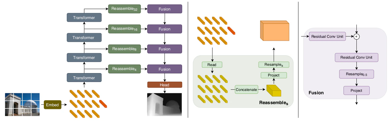
DPTの処理の流れ
DPTの処理の流れの大枠は上図より確認することができます。詳しい処理については以下で確認します。
Transformer Encoder
Transformerに基づくEncoderではまずEmbedding処理を行うことで下記のようなテンソルを取得します。
\begin{align}
t^0 &= \{ t_0^0, \cdots , t_{N_p}^0 \} \\
t_n^0 & \in \mathbb{R}^{D} \\
N_p &= \frac{WH}{p^{2}}
\end{align}
上記の$t^0$の$0$はTransformerの$0$層(入力)であると解釈すると良いです。$p$はパッチサイズでありDPTではオリジナルのViTと同様に$p=16$が用いられます。
また、DPT論文では下記のような3種類のネットワーク構造を用いて検証が行われている点も合わせて抑えておくと良いです。
| ネットワークの名称 | 実行される処理 |
|---|---|
ViT-Base |
patch-based Embedding + 12層のTransformer |
ViT-Large |
patch-based Embedding + 24層のTransformer |
ViT-Hybrid |
ResNet50を用いたEmbedding + 12層のTransformer |
Convolutional Decoder
\begin{align}
\mathrm{Reassemble}_{s}^{\hat{D}}(t) = (\mathrm{Resample}_{s} \circ \mathrm{Concatenate} \circ \mathrm{Read})(t)
\end{align}
Convolutional Decoderでは上記のような3段階の処理が行われます。以下、それぞれについて詳しく確認します。
\begin{align}
\mathrm{Read}: \, \mathbb{R}^{(N_p + 1) \times D} \longrightarrow \mathbb{R}^{N_p \times D}
\end{align}
まず$\mathrm{Read}$では上記のようにトークンの数を$N_{p}+1$個から$N_{p}$個に減らす処理を行います(ViTなどではパッチに基づくトークン以外にもう1つトークンを持つように実装されている)。実装方法は様々ですが、たとえば下記の3通りの方法などが挙げられます。
\begin{align}
\mathrm{Read}_{\mathrm{ingore}}(t) &= \{ t_1, \cdots , t_{N_p} \} \\
\mathrm{Read}_{\mathrm{add}}(t) &= \{ t_1+t_0, \cdots , t_{N_p}+t_0 \} \\
\mathrm{Read}_{\mathrm{proj}}(t) &= \{ \mathrm{MLP}(\mathrm{concat}(t_1,t_0)), \cdots , \mathrm{MLP}(\mathrm{concat}(t_{N_p},t_0)) \}
\end{align}
上記はそれぞれ「$t_0$の特徴量を用いない(ignore)」、「他のトークンに加える(add)」、「concatで連結した後にMLPで元の次元に戻す(proj)」のように理解すると良いです。
次に$\mathrm{Concatenate}$ではTransformerの1Dのトークンを画像に対応するように2Dに配置します。
\begin{align}
\mathrm{Concatenate} &: \, \mathbb{R}^{N_p \times D} \longrightarrow \mathbb{R}^{\frac{W}{p} \times \frac{H}{p} \times D} \\
N^{p} &= \frac{WH}{p^2}
\end{align}
$\mathrm{Resample}$処理では$1 \times 1$畳み込みによってチャネルの数を$D \rightarrow \hat{D}$に変えた後にリサンプリングを行います。
\begin{align}
\mathrm{Resample}_s & : \, \mathbb{R}^{\frac{W}{p} \times \frac{H}{p} \times D} \longrightarrow \mathbb{R}^{\frac{W}{s} \times \frac{H}{s} \times \hat{D}} \\
\hat{D} &= 256 \qquad \mathrm{(Default} \, \mathrm{Architecture)}
\end{align}
上記のような処理を行うことで複数の解像度の特徴マップを構築することができます。また、下記の表では3種類のDPTにおけるReassemble処理を行うViTのlayerについてまとめました。
| ネットワークの名称 | Reassemble処理を行うViTのlayer |
|---|---|
DPT-Base |
5, 12, 18, 24 |
DPT-Large |
3, 6, 9, 12 |
DPT-Hybrid |
9, 12 |
DPTの実装
当節では上記で確認を行ったVGGTの実装におけるDPTの実装について確認します。
class DPTHead(nn.Module):
    """
    DPT  Head for dense prediction tasks.

    This implementation follows the architecture described in "Vision Transformers for Dense Prediction"
    (https://arxiv.org/abs/2103.13413). The DPT head processes features from a vision transformer
    backbone and produces dense predictions by fusing multi-scale features.

    Args:
        dim_in (int): Input dimension (channels).
        patch_size (int, optional): Patch size. Default is 14.
        output_dim (int, optional): Number of output channels. Default is 4.
        activation (str, optional): Activation type. Default is "inv_log".
        conf_activation (str, optional): Confidence activation type. Default is "expp1".
        features (int, optional): Feature channels for intermediate representations. Default is 256.
        out_channels (List[int], optional): Output channels for each intermediate layer.
        intermediate_layer_idx (List[int], optional): Indices of layers from aggregated tokens used for DPT.
        pos_embed (bool, optional): Whether to use positional embedding. Default is True.
        feature_only (bool, optional): If True, return features only without the last several layers and activation head. Default is False.
        down_ratio (int, optional): Downscaling factor for the output resolution. Default is 1.
    """

    def __init__(
        self,
        dim_in: int,
        patch_size: int = 14,
        output_dim: int = 4,
        activation: str = "inv_log",
        conf_activation: str = "expp1",
        features: int = 256,
        out_channels: List[int] = [256, 512, 1024, 1024],
        intermediate_layer_idx: List[int] = [4, 11, 17, 23],
        pos_embed: bool = True,
        feature_only: bool = False,
        down_ratio: int = 1,
    ) -> None:
        super(DPTHead, self).__init__()
        self.patch_size = patch_size
        self.activation = activation
        self.conf_activation = conf_activation
        self.pos_embed = pos_embed
        self.feature_only = feature_only
        self.down_ratio = down_ratio
        self.intermediate_layer_idx = intermediate_layer_idx

        self.norm = nn.LayerNorm(dim_in)

        ...

    def forward(
        self,
        aggregated_tokens_list: List[torch.Tensor],
        images: torch.Tensor,
        patch_start_idx: int,
        frames_chunk_size: int = 8,
    ) -> Union[torch.Tensor, Tuple[torch.Tensor, torch.Tensor]]:
        """
        Forward pass through the DPT head, supports processing by chunking frames.
        Args:
            aggregated_tokens_list (List[Tensor]): List of token tensors from different transformer layers.
            images (Tensor): Input images with shape [B, S, 3, H, W], in range [0, 1].
            patch_start_idx (int): Starting index for patch tokens in the token sequence.
                Used to separate patch tokens from other tokens (e.g., camera or register tokens).
            frames_chunk_size (int, optional): Number of frames to process in each chunk.
                If None or larger than S, all frames are processed at once. Default: 8.

        Returns:
            Tensor or Tuple[Tensor, Tensor]:
                - If feature_only=True: Feature maps with shape [B, S, C, H, W]
                - Otherwise: Tuple of (predictions, confidence) both with shape [B, S, 1, H, W]
        """
        B, S, _, H, W = images.shape

        # If frames_chunk_size is not specified or greater than S, process all frames at once
        if frames_chunk_size is None or frames_chunk_size >= S:
            return self._forward_impl(aggregated_tokens_list, images, patch_start_idx)

        # Otherwise, process frames in chunks to manage memory usage
        assert frames_chunk_size > 0

        # Process frames in batches
        all_preds = []
        all_conf = []

        for frames_start_idx in range(0, S, frames_chunk_size):
            frames_end_idx = min(frames_start_idx + frames_chunk_size, S)

            # Process batch of frames
            if self.feature_only:
                chunk_output = self._forward_impl(
                    aggregated_tokens_list, images, patch_start_idx, frames_start_idx, frames_end_idx
                )
                all_preds.append(chunk_output)
            else:
                chunk_preds, chunk_conf = self._forward_impl(
                    aggregated_tokens_list, images, patch_start_idx, frames_start_idx, frames_end_idx
                )
                all_preds.append(chunk_preds)
                all_conf.append(chunk_conf)

        # Concatenate results along the sequence dimension
        if self.feature_only:
            return torch.cat(all_preds, dim=1)
        else:
            return torch.cat(all_preds, dim=1), torch.cat(all_conf, dim=1)
上記よりメイン処理はself._forward_impl内で行われていることが確認できます。
class DPTHead(nn.Module):
    def __init__(
        self,
        dim_in: int,
        patch_size: int = 14,
        output_dim: int = 4,
        activation: str = "inv_log",
        conf_activation: str = "expp1",
        features: int = 256,
        out_channels: List[int] = [256, 512, 1024, 1024],
        intermediate_layer_idx: List[int] = [4, 11, 17, 23],
        pos_embed: bool = True,
        feature_only: bool = False,
        down_ratio: int = 1,
    ) -> None:
        super(DPTHead, self).__init__()
        self.patch_size = patch_size
        self.activation = activation
        self.conf_activation = conf_activation
        self.pos_embed = pos_embed
        self.feature_only = feature_only
        self.down_ratio = down_ratio
        self.intermediate_layer_idx = intermediate_layer_idx

        self.norm = nn.LayerNorm(dim_in)

        # Projection layers for each output channel from tokens.
        self.projects = nn.ModuleList(
            [nn.Conv2d(in_channels=dim_in, out_channels=oc, kernel_size=1, stride=1, padding=0) for oc in out_channels]
        )

    ...

    def _forward_impl(
        self,
        aggregated_tokens_list: List[torch.Tensor],
        images: torch.Tensor,
        patch_start_idx: int,
        frames_start_idx: int = None,
        frames_end_idx: int = None,
    ) -> Union[torch.Tensor, Tuple[torch.Tensor, torch.Tensor]]:
        """
        Implementation of the forward pass through the DPT head.

        This method processes a specific chunk of frames from the sequence.

        Args:
            aggregated_tokens_list (List[Tensor]): List of token tensors from different transformer layers.
            images (Tensor): Input images with shape [B, S, 3, H, W].
            patch_start_idx (int): Starting index for patch tokens.
            frames_start_idx (int, optional): Starting index for frames to process.
            frames_end_idx (int, optional): Ending index for frames to process.

        Returns:
            Tensor or Tuple[Tensor, Tensor]: Feature maps or (predictions, confidence).
        """
        if frames_start_idx is not None and frames_end_idx is not None:
            images = images[:, frames_start_idx:frames_end_idx].contiguous()

        B, S, _, H, W = images.shape

        patch_h, patch_w = H // self.patch_size, W // self.patch_size

        out = []
        dpt_idx = 0

        for layer_idx in self.intermediate_layer_idx:
            x = aggregated_tokens_list[layer_idx][:, :, patch_start_idx:]

            # Select frames if processing a chunk
            if frames_start_idx is not None and frames_end_idx is not None:
                x = x[:, frames_start_idx:frames_end_idx]

            x = x.reshape(B * S, -1, x.shape[-1])
            x = self.norm(x)
            x = x.permute(0, 2, 1).reshape((x.shape[0], x.shape[-1], patch_h, patch_w))
            x = self.projects[dpt_idx](x)

            if self.pos_embed:
                x = self._apply_pos_embed(x, W, H)

            x = self.resize_layers[dpt_idx](x)

            out.append(x)
            dpt_idx += 1

        # Fuse features from multiple layers.
        out = self.scratch_forward(out)
        # Interpolate fused output to match target image resolution.
        out = custom_interpolate(
            out,
            (int(patch_h * self.patch_size / self.down_ratio), int(patch_w * self.patch_size / self.down_ratio)),
            mode="bilinear",
            align_corners=True,
        )

        if self.pos_embed:
            out = self._apply_pos_embed(out, W, H)

        if self.feature_only:
            return out.view(B, S, *out.shape[1:])

        out = self.scratch.output_conv2(out)
        preds, conf = activate_head(out, activation=self.activation, conf_activation=self.conf_activation)

        preds = preds.view(B, S, *preds.shape[1:])
        conf = conf.view(B, S, *conf.shape[1:])
        return preds, conf
上記のfor layer_idx in self.intermediate_layer_idx:のループ内で[4, 11, 17, 23]層からそれぞれ特徴量を抽出し、リシェイプや正規化処理を行っている点に着目しておくと良いです。複数のレイヤーの特徴量の混ぜ合わせについてはout = self.scratch_forward(out)で実行されます。
class DPTHead(nn.Module):
    def __init__(
        self,
        dim_in: int,
        patch_size: int = 14,
        output_dim: int = 4,
        activation: str = "inv_log",
        conf_activation: str = "expp1",
        features: int = 256,
        out_channels: List[int] = [256, 512, 1024, 1024],
        intermediate_layer_idx: List[int] = [4, 11, 17, 23],
        pos_embed: bool = True,
        feature_only: bool = False,
        down_ratio: int = 1,
    ) -> None:
        super(DPTHead, self).__init__()
        self.patch_size = patch_size
        self.activation = activation
        self.conf_activation = conf_activation
        self.pos_embed = pos_embed
        self.feature_only = feature_only
        self.down_ratio = down_ratio
        self.intermediate_layer_idx = intermediate_layer_idx

        self.norm = nn.LayerNorm(dim_in)

        # Projection layers for each output channel from tokens.
        self.projects = nn.ModuleList(
            [nn.Conv2d(in_channels=dim_in, out_channels=oc, kernel_size=1, stride=1, padding=0) for oc in out_channels]
        )

        ...

        self.scratch = _make_scratch(out_channels, features, expand=False)

        # Attach additional modules to scratch.
        self.scratch.stem_transpose = None
        self.scratch.refinenet1 = _make_fusion_block(features)
        self.scratch.refinenet2 = _make_fusion_block(features)
        self.scratch.refinenet3 = _make_fusion_block(features)
        self.scratch.refinenet4 = _make_fusion_block(features, has_residual=False)

        ...

    ...

    def scratch_forward(self, features: List[torch.Tensor]) -> torch.Tensor:
        """
        Forward pass through the fusion blocks.

        Args:
            features (List[Tensor]): List of feature maps from different layers.

        Returns:
            Tensor: Fused feature map.
        """
        layer_1, layer_2, layer_3, layer_4 = features

        layer_1_rn = self.scratch.layer1_rn(layer_1)
        layer_2_rn = self.scratch.layer2_rn(layer_2)
        layer_3_rn = self.scratch.layer3_rn(layer_3)
        layer_4_rn = self.scratch.layer4_rn(layer_4)

        out = self.scratch.refinenet4(layer_4_rn, size=layer_3_rn.shape[2:])
        del layer_4_rn, layer_4

        out = self.scratch.refinenet3(out, layer_3_rn, size=layer_2_rn.shape[2:])
        del layer_3_rn, layer_3

        out = self.scratch.refinenet2(out, layer_2_rn, size=layer_1_rn.shape[2:])
        del layer_2_rn, layer_2

        out = self.scratch.refinenet1(out, layer_1_rn)
        del layer_1_rn, layer_1

        out = self.scratch.output_conv1(out)
        return out
scratch_forwardメソッドで出てくるRefineNetの実装についてはDepthAnythingの実装を元に下記でも取り扱ったので合わせてご確認ください。