TL;DR
- fastprogressを使うと、Deep Learningのモデルを学習させるとき自動で色々なものを出力してくれてすごく便利
- 特にjupyter上で学習を回すときにはとても良さそう
- 実際にfastprogressを使って学習を回すと以下のような感じになる

(fastai/fastprogress: Simple and flexible progress bar for Jupyter Notebook and console より)
fastprogressでできること
- 1エポックごとに、損失関数とかmetricsの値を標準出力に出力させたい
- 学習の進み具合を示すプログレスバーを、上記の標準出力と喧嘩しない形で表示させたい
- できればリアルタイムで学習曲線の表示もしてほしい...
fastprogressを用いると全部実現可能。
これを使えば、少なくともDeep Learningのモデル学習時には、tqdmとかprintとかに用はなくなると思われる。
公式
githubのURLは以下。
fastai/fastprogress: Simple and flexible progress bar for Jupyter Notebook and console
インストール
pipでインストール可能
$ pip install fastprogress
基本的な使い方
基本的に、Deep Learningの学習の合間合間に、fastprogressを用いた出力のための処理を挟むだけである。
from fastprogress import master_bar, progress_bar


n_epochs = 20  # エポック数
b_batches = 10  # 1エポックあたりのバッチ数

x_bounds = [0, n_epochs]  # 表示させる学習曲線の図のx軸の範囲
y_bounds = [0, 1]         # 表示させる学習曲線の図のy軸の範囲

mb = master_bar(range(n_epochs))
for i in mb:  # エポックに関するイテレーション
    for j in progress_bar(range(n_batches), parent=mb):  # バッチに関するイテレーション
        # バッチごとの学習処理を記述
        train(x_batch, y_batch)

    graphs = ...   # グラフに関する設定
    mb.update_graph(graphs, x_bounds, y_bounds)  # 1エポックごとにグラフのアップデート
    mb.write('comment')  # ここに、1エポックごとに出力させたい内容を書く
使用例
mnistの画像を分類する2層ニューラルネットをtensorflowで構築し、fastprogressを用いて学習の様子を表示するスクリプトを作成した。
import numpy as np
from fastprogress import master_bar, progress_bar


def training(session, training_op, cost, train_data, valid_data,
             y_upper_bound=None, seed=0, n_epochs=10, batch_size=128):
    """
    * train_data
    * valid_data
    はいずれも、
    * key : tensorflowのplaceholder
    * val : numpyのarray(全データ)
    のディクショナリ形式で与える
    """
    np.random.seed(seed)

    # バッチ数を計算
    n_samples_train = len(list(train_data.values())[0])
    n_samples_valid = len(list(valid_data.values())[0])
    n_batches_train = n_samples_train//batch_size
    n_batches_valid = n_samples_valid//batch_size
    mb = master_bar(range(n_epochs))

    # 学習曲線描画のための前準備
    train_costs_lst = []
    valid_costs_lst = []
    x_bounds = [0, n_epochs]
    y_bounds = None
    for epoch in mb:
        # Train
        train_costs = []
        for _ in progress_bar(range(n_batches_train), parent=mb):
            batch_idx = np.random.randint(n_samples_train, size=batch_size)

            # feedするデータを指定
            feed_dict = {}
            for k, v in train_data.items():
                feed_dict[k] = v[batch_idx]

            _, train_cost = session.run(
                [training_op, cost], feed_dict=feed_dict)
            train_costs.append(train_cost)

        # Valid
        valid_costs = []
        for i in range(n_batches_valid):
            start = i * batch_size
            end = start + batch_size

            # feedするデータを指定
            feed_dict = {}
            for k, v in valid_data.items():
                feed_dict[k] = v[start:end]

            valid_cost = session.run(cost, feed_dict=feed_dict)
            valid_costs.append(valid_cost)

        # 損失関数の値の計算
        train_costs_mean = np.mean(train_costs)
        valid_costs_mean = np.mean(valid_costs)
        train_costs_lst.append(train_costs_mean)
        valid_costs_lst.append(valid_costs_mean)

        # learning curveの図示
        if y_bounds is None:
            # 1エポック目のみ実行
            y_bounds = [0, train_costs_mean *
                        1.1 if y_upper_bound is None else y_upper_bound]

        t = np.arange(len(train_costs_lst))
        graphs = [[t, train_costs_lst], [t, valid_costs_lst]]
        mb.update_graph(graphs, x_bounds, y_bounds)

        # 学習過程の出力
        mb.write('EPOCH: {0:02d}, Training cost: {1:10.5f}, Validation cost: {2:10.5f}'.format(
            epoch+1, train_costs_mean, valid_costs_mean))


if __name__ == '__main__':
    import tensorflow as tf
    from keras.datasets import mnist
    from sklearn.model_selection import train_test_split
    from sklearn.metrics import accuracy_score

    # mnistデータのロード
    (x_train, y_train), (x_test, y_test) = mnist.load_data()

    # 学習用データ(更に学習用と検証用とに分ける)
    x_train = x_train.reshape(-1, 784) / 255
    x_train, x_valid, y_train, y_valid = train_test_split(
        x_train, y_train, test_size=0.1, random_state=42)

    # テスト用データ
    x_test = x_test.reshape(-1, 784) / 255

    # ネットワークの構築
    # 2層ニューラルネット
    # 中間層のノード数は50, activationはRelu
    tf.set_random_seed(0)
    X = tf.placeholder(shape=(None, 784), dtype=tf.float32)
    y = tf.placeholder(shape=(None, ), dtype=tf.int32)
    hidden = tf.keras.layers.Dense(50, activation='relu')(X)
    logits = tf.keras.layers.Dense(10, activation=None)(hidden)
    cost = tf.nn.sparse_softmax_cross_entropy_with_logits(
        logits=logits, labels=y)
    training_op = tf.train.AdamOptimizer().minimize(cost)

    # 学習
    session = tf.Session()
    session.run(tf.global_variables_initializer())
    training(session=session, training_op=training_op, cost=cost,
             train_data={X: x_train, y: y_train}, valid_data={X: x_valid, y: y_valid},
             y_upper_bound=None, n_epochs=10, batch_size=128)

    # 学習精度の検証
    pred = np.argmax(logits.eval(
        session=session, feed_dict={X: x_test}), axis=1)
    print(accuracy_score(y_test,  pred))
    session.close()
結果は以下の通りとなった。
Total time: 00:11
EPOCH: 01, Training cost: 0.45633, Validation cost: 0.25553

EPOCH: 02, Training cost: 0.21853, Validation cost: 0.19071

EPOCH: 03, Training cost: 0.16616, Validation cost: 0.16419

EPOCH: 04, Training cost: 0.14049, Validation cost: 0.14273

EPOCH: 05, Training cost: 0.12066, Validation cost: 0.13515

EPOCH: 06, Training cost: 0.10547, Validation cost: 0.12264

EPOCH: 07, Training cost: 0.09498, Validation cost: 0.11546

EPOCH: 08, Training cost: 0.08215, Validation cost: 0.10997

EPOCH: 09, Training cost: 0.07280, Validation cost: 0.10653

EPOCH: 10, Training cost: 0.06529, Validation cost: 0.10137
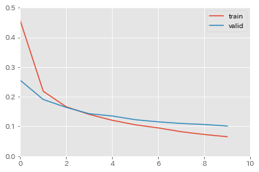
10エポックの学習が完了。
学習用・検証用それぞれのデータに対する損失関数の値をいい感じに出力・図示してくれている。
実際の学習時には、
- 学習全体
- エポック毎
のプログレスバーが表示され、学習曲線の図はリアルタイムに更新されていく(プログレスバーは、100%になると自動的に画面から消える)。
(どうやら、表示される学習曲線のグラフのlegendは、デフォルトだと1つ目がtrain、2つ目がvalidとなってくれる模様。)