GeForce GTX 1070 (8GB)
ASRock Z170M Pro4S [Intel Z170chipset]
Ubuntu 16.04 LTS desktop amd64
TensorFlow v1.2.1
cuDNN v5.1 for Linux
CUDA v8.0
Python 3.5.2
IPython 6.0.0 -- An enhanced Interactive Python.
gcc (Ubuntu 5.4.0-6ubuntu1~16.04.4) 5.4.0 20160609
GNU bash, version 4.3.48(1)-release (x86_64-pc-linux-gnu)
scipy v0.19.1
geopandas v0.3.0
MATLAB R2017b (Home Edition)
ADDA v.1.3b6
Introduction
The light scattering properties of a single particle is a fundamental value used in the numerical simulation of the cometary dust (Kolokolova et al., 2004), regolith on the Asteroid (Levasseur-Regourd and Hadamcik, 2003; Hasselmann et al., 2017), atmospheric aerosols (Chakrabarty et al., 2014), atmospheric ice crystals (Masuda and Ishimoto, 2017), and microbio cells (Yurkin 2007).
Every single particle of the above mentioned particles is non-spherical (see SEM images of the samples in the Summary in Amsterdam-Granada light scattering database, for example). It is well known that the light scattering properties of the spherical and non-spherical particles are totally different, resulting in the totally different results in the numerical simulations mentioned above (Mishchenko et al., 2000).
However, the computation of the light scattering properties of the non-spherical particles are still challenging and requires the much larger computation time even by using the state-of-the-art supercomputers. With the advent of the GPU (the Graphics Processing Unit), those computations becomes in parallel reducing the wall time of the computation.
Still, there is the demand to improve the computation efficiencies in the non-spherical light scattering simulation considering that the non-spherical particles have the different properties to investigate (e.g. surface roughness, outer shape, elongation, structure such as aggregates, and mixture of materials).
In the numerical light scattering simulation, the random orientation averaging is often performed to obtain the averaging properties of the non-spherical particles. In this article, the computation of the numerical orientation averaging are compared for the three different method to obtain the point sets over the spherical surface.
Numerical orientation averaging
The number of point sets over the sphere
In order to obtain the light scattering properties of non-spherical particles with random orientations, there are two methods:
- Analytical orientation averaging (AOA)
- Numerical orientation averaging (NOA)
The AOA such as T-matrix method (Mishchenko et al., 2017), is rigorous and accurate. However, for the particle shape having difficulty to obtain analytical solution (e.g. the T-matrix), the NOA is the method to perform the simulation.
For the NOA, the number of orientations to perform the averaging is the key parameter. The computation time to perform numerical simulations is proportional to the number of orientations. Therefore, reducing the number of orientations leads to the reducing the computation time in the numerical simulations. For this, different orientation averaging schemes have been studied to obtain efficient method for the numerical simulations (see Okada(2008), Pentilla et al. (2011), Um and McFarquhar (2013) and Zhang (2018)).
Hardin et al. (2016) studied the comparison of popular point configuration on the spherical surface:$S^2$.
Their study is directly related to the NOA in our simulations. It is interesting to investigate the efficiencies of the different point sets over the $S^2$ to obtain the light scattering properties of the non-spherical particles.
The spherepts package (MATLAB)
In Hardin et al.(2016), the Matlab code to implement different points sets is introduced (Section 5). The Matlab code is named "spherepts" developed by Grady Wright.
By using the spherepts, following point sets on the sphere can be obtained.
- Icosahedral Nodes
- Cubed Nodes
- HEALPix
- Fibonacci Nodes
- Minimum energy Nodes
- Maximum determination Nodes
- Symmetric t-design Nodes
- Hammersley Nodes
The pySpherepts package (Python + Numpy + Scipy)
The spherepts package implemented in the Matlab is useful to perform numerical orientation averaging. However, in the system using Python (and Numpy) for data analysis, it is more portable to have those process in the Python (and Numpy) implementation.
Some of the spherepts implementation for Matlab are ported to those in Python (and Numpy, Scipy) implementation. The package is named the "pySpherepts".
In pySpherepts package (as of Feb. 17, 2018), following point sets have been ported:
- Icosahedral Nodes
- Fibonacci nodes
- Hammersley nodes
In this article, the pySpherepts is used to obtain particle orientations for the above three point sets.
The orientation averaging for the beta and gamma (fixed alpha=0.0)
In this article, light scattering simulation code ADDA is used (Yurkin and Hoekstra, 2007).
The light scattering properties is defined for the three Euler angles (alpha, beta and gamma). The ADDA uses "zyz-notation" or "y-convention" (see 8.1 Single orientation in Yurkin and Hoekstra, 2014).
In ADDA, the rotation over the alpha is equivalent to rotating the scattering plane without changing the orientation of the particle relative to the incident light (see 8.2 Orientation averaging in Yurkin and Hoekstra, 2014).
In this article, orientation averaging is performed for the beta and the gamma. It is noted that the alpha is fixed as 0.0. However, for the study of the light scattering properties, it is normal to perform averaging also for the alpha, which will require increased computation time by the $N_{alpha}$ factor for the numerical simulations, where the $N_{alpha}$ is the number of orientations for the alpha.
Calculation
Particle shape
The axisymmetric Chebyshev particle is used for the particle shape.
r = r_0 [ 1 + \epsilon cos(n\theta) ]
Following parameter is used:
-shape chebyshev 0.7 12
where eps=0.7 and n=12.
The Figure 1 shows the particle shape rendered using POV-Ray.

Fig. 1. The particle shape used in the simulation from the different viewing angles. Colors represent the X position of the dipoles to improve the visualization in 3 dimension.
Simulation parameters
Following parameters are used for the numerical simulation.
Table 1. Simulation parameters
Generated by ADDA v.1.3b6
command: './adda -orient 0.0 132.819 178.2 -ntheta 180 -grid 104 -shape chebyshev 0.7 12 -m 1.5 0.005 -eq_rad 6.299605 -store_int_field '
lambda: 6.283185307
shape: axisymmetric chebyshev particle; size along x-axis (Dx):17.88632149, amplitude eps=0.7, order n=12, initial radius r0/Dx=0.2941176471
box dimensions: 104x104x104
refractive index: 1.5+0.005i
Dipoles/lambda: 36.5893
	(Volume correction used)
Required relative residual norm: 1e-05
Total number of occupied dipoles: 206800
Volume-equivalent size parameter: 6.299605
...
Results
Relative error
Relative error is defined as follows:
Err(\%) = \frac{|A-B|}{B} * 100
In this article, B is taken from the results for the Icosahedral Nodes having N=2562.
Qext and Qabs
Figure 2 shows the Qext and Qabs as a function of the number of orientations (i.e. Nori). Results are for Hammersley Nodes, Icosahedral Nodes, and Fibonacci Nodes in blue, red, and green, respectively.
Values of the Qext and Qabs are shown in Table 2-1 through Table 3-3. As shown in the tables, the relative errors in the Qext and Qabs become less than 1.0 % when the Nori exceeds 500.
The difference in the orientation averaging efficiencies for the Qext and Qabs among the three point sets is not remarkable.

Fig. 2. Qext and Qabs as a function of the number of the orientations. The blue, red and green marks represent (b)Hammersley Nodes, (r)Icosahedral Nodes, and (g)Fibonacci Nodes, respectively.
Table 2-1. Qext and relative error for HN (Hammersley Nodes). The B is Qext(IN) having Nori=2562.
| Nori | A: Qext(HN) | abs(A - B) / B * 100 |
|---|---|---|
| 30 | 4.5541695 | 0.6518 |
| 60 | 4.5345399 | 0.2179 |
| 100 | 4.5249185 | 0.0053 |
| 300 | 4.5257659 | 0.0240 |
| 500 | 4.5247191 | 0.0009 |
| 1000 | 4.5244589 | 0.0049 |
| 1500 | 4.5245262 | 0.0034 |
| 2000 | 4.5242891 | 0.0086 |
Table 2-2. Same as Table 2-1 but for Qext(IN): Icosahedral Nodes. The B is Qext(IN) having Nori=2562.
| Nori | A: Qext(IN) | abs(A - B) / B * 100 |
|---|---|---|
| 12 | 4.5058261 | 0.4167 |
| 42 | 4.5469316 | 0.4918 |
| 162 | 4.5290211 | 0.0960 |
| 642 | 4.5255275 | 0.0187 |
| 2562 | 4.5246793 | --- |
Table 2-3. Same as Table 2-1 but for Qext(FN): Fibonacci Nodes. The B is Qext(IN) having Nori=2562.
| Nori | A: Qext(FN) | abs(A - B) / B * 100 |
|---|---|---|
| 31 | 4.5240969 | 0.0129 |
| 61 | 4.5241208 | 0.0123 |
| 101 | 4.5241406 | 0.0119 |
| 301 | 4.5241157 | 0.0125 |
| 501 | 4.524116 | 0.0124 |
| 1001 | 4.524115 | 0.0125 |
| 1501 | 4.5241154 | 0.0125 |
| 2001 | 4.5241153 | 0.0125 |
Table 3-1. Qabs and relative error for HN (Hammersley Nodes). The B is Qabs(IN) having Nori=2562.
| Nori | A: Qabs(HN) | abs(A - B) / B * 100 |
|---|---|---|
| 30 | 0.1299081 | 0.2695 |
| 60 | 0.1296061 | 0.0364 |
| 100 | 0.1297289 | 0.1312 |
| 300 | 0.1296017 | 0.0330 |
| 500 | 0.1296158 | 0.0439 |
| 1000 | 0.1296013 | 0.0327 |
| 1500 | 0.1295918 | 0.0254 |
| 2000 | 0.1295939 | 0.0270 |
Table 3-2. Same as Table 3-1 but for Qabs(IN): Icosahedral Nodes. The B is Qabs(IN) having Nori=2562.
| Nori | A: Qabs(IN) | abs(A - B) / B * 100 |
|---|---|---|
| 12 | 0.1300914 | 0.4110 |
| 42 | 0.1298414 | 0.2180 |
| 162 | 0.1296391 | 0.0619 |
| 642 | 0.1295761 | 0.0133 |
| 2562 | 0.1295589 | --- |
Table 3-3. Same as Table 3-1 but for Qabs(FN): Fibonacci Nodes. The B is Qabs(IN) having Nori=2562.
| Nori | A: Qabs(FN) | abs(A - B) / B * 100 |
|---|---|---|
| 31 | 0.1296488 | 0.0694 |
| 61 | 0.1296038 | 0.0347 |
| 101 | 0.1295946 | 0.0276 |
| 301 | 0.129589 | 0.0232 |
| 501 | 0.1295885 | 0.0228 |
| 1001 | 0.1295883 | 0.0227 |
| 1501 | 0.1295883 | 0.0227 |
| 2001 | 0.1295883 | 0.0227 |
Phase function and Degree of polarization
Figure 3 shows the phase function and the Degree of polarization for Hammersley Nodes having different values of the number of orientations (Nori) in the full length of the scattering angles, and those in the backward scattering.
Figure 4 are the phase function and degree of polarization as a function of the number of orientations (NOri). Results are for Hammersley Nodes, Icosahedral Nodes, and Fibonacci Nodes in blue, red, and green, respectively.
As shown in the figure, as the number of orientations increases, the values of the phase functions and those of the polarization converge.
Table 4-1 through Table 5-3 show the values and relative errors for the different point sets. It is shown that the relative errors become less than 1% when the number of orientations exceeds 500.
The difference in the orientation averaging efficiencies for the S11 and Pol among the three point sets is not remarkable.
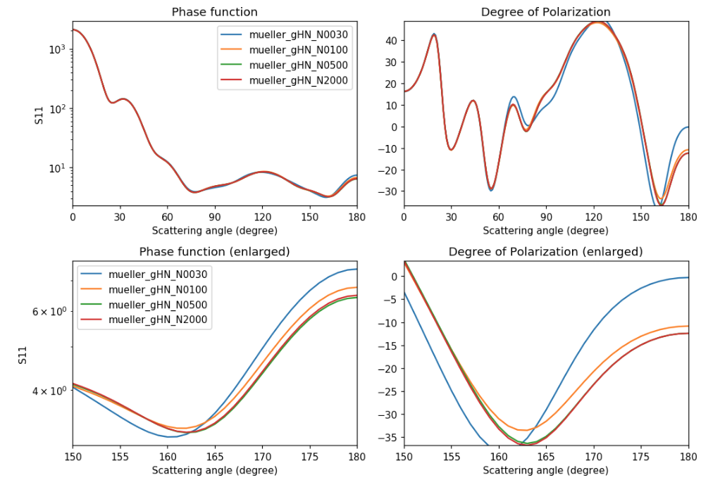
Fig. 3. Phase function and Degree of polarization as a function of scattering angle, rendered by showMueller_180113.ipynb v0.7. The upper panels show the results in the full length of the scattering angle. The lower panels show the results in the scattering angles related to the negative polarization branch shown for the cometary dust.

Fig. 4. Phase function and Degree of polarization as a function of the number of orientations. The blue, red and green marks represent (b)Hammersley Nodes, (r)Icosahedral Nodes, and (g)Fibonacci Nodes, respectively.
Table 4-1. Phase function and relative error for HN (Hammersley Nodes). The B is S11(IN) having Nori=2562. The scattering angle is 170 degree.
| Nori | A: S11(HN) | abs(A - B) / B * 100 |
|---|---|---|
| 30 | 4.94326 | 12.7739 |
| 60 | 4.536754 | 3.5001 |
| 100 | 4.58954 | 4.7043 |
| 300 | 4.444392 | 1.3929 |
| 500 | 4.349006 | 0.7832 |
| 1000 | 4.377727 | 0.1279 |
| 1500 | 4.382704 | 0.0144 |
| 2000 | 4.390335 | 0.1597 |
Table 4-2. Same as Table 4-1 but for S11(IN): Icosahedral Nodes. The B is S11(IN) having Nori=2562. The scattering angle is 170 degree.
| Nori | A: S11(IN) | abs(A - B) / B * 100 |
|---|---|---|
| 12 | 2.329375 | 46.8584 |
| 42 | 5.006174 | 14.2092 |
| 162 | 4.328343 | 1.2546 |
| 642 | 4.382297 | 0.0237 |
| 2562 | 4.383335 | --- |
Table 4-3. Same as Table 4-1 but for S11(FN): Fibonacci Nodes. The B is S11(IN) having Nori=2562. The scattering angle is 170 degree.
| Nori | A: S11(FN) | abs(A - B) / B * 100 |
|---|---|---|
| 31 | 4.104669 | 6.3574 |
| 61 | 4.270889 | 2.5653 |
| 101 | 4.351807 | 0.7193 |
| 301 | 4.392717 | 0.2140 |
| 501 | 4.396591 | 0.3024 |
| 1001 | 4.398315 | 0.3417 |
| 1501 | 4.398605 | 0.3484 |
| 2001 | 4.398712 | 0.3508 |
Table 5-1. Degree of polarization and relative error for HN (Hammersley Nodes). The B is Pol(IN) having Nori=2562. The scattering angle is 170 degree.
| Nori | A: Pol(HN) | abs(A - B) / B * 100 |
|---|---|---|
| 30 | -11.7412598164 | 50.1332 |
| 60 | -15.8224580835 | 32.7997 |
| 100 | -20.7454559716 | 11.8910 |
| 300 | -22.6421296771 | 3.8356 |
| 500 | -23.5499560129 | 0.0201 |
| 1000 | -23.6671679161 | 0.5179 |
| 1500 | -23.5305418755 | 0.0624 |
| 2000 | -23.5956253908 | 0.2141 |
Table 5-2. Same as Table 5-1 but for Pol(IN): Icosahedral Nodes. The B is Pol(IN) having Nori=2562. The scattering angle is 170 degree.
| Nori | A: Pol(IN) | abs(A - B) / B * 100 |
|---|---|---|
| 12 | -32.4526965388 | 37.8313 |
| 42 | -20.9038079779 | 11.2185 |
| 162 | -22.0221687607 | 6.4686 |
| 642 | -23.5953656267 | 0.2130 |
| 2562 | -23.5452229866 | --- |
Table 5-3. Same as Table 5-1 but for Pol(FN): Fibonacci Nodes. The B is Pol(IN) having Nori=2562. The scattering angle is 170 degree.
| Nori | A: Pol(FN) | abs(A - B) / B * 100 |
|---|---|---|
| 31 | -27.128399391 | 15.2183 |
| 61 | -26.230112747 | 11.4031 |
| 101 | -24.5505602615 | 4.2698 |
| 301 | -23.5750447844 | 0.1267 |
| 501 | -23.4863556788 | 0.2500 |
| 1001 | -23.4478203585 | 0.4137 |
| 1501 | -23.4405453547 | 0.4446 |
| 2001 | -23.4379518368 | 0.4556 |
Summary
In this article, following three point sets are studied for the efficiencies in the random orientation averaging of the light scattering properties of the non-spherical particles (Chebyshev particle).
- Hammersley Nodes
- Icosahedral Nodes
- Fibonacci Nodes
Extinction and absorption efficiencies, phase function and degree of polarization are investigated.
It is shown that all the three point sets show the behavior of the convergence as the number of orientations increases.
The difference in the orientation averaging efficiencies among the three point sets is not noticeable when the number of orientations exceeds 500.
Reference
- D.P. Hardin, T. Michaels, and E. B. Staff, A Comparison of Popular Configurations on S^2, Dolomites Resaerch Notes on Approximation, 9, 16-49, 2016.
- M. I. Mishchenko, N. T. Zakharova, N. G. Khlebtsov, G. Videen, and T. Wriedt,
Comprehensive thematic T-matrix reference database: a 2015-2017 update., J. Quant. Spectrosc. Radiat. Transf., 202, 240-246, 2017 - J. Reeger and B. Fornbeg, Numerical Quadrature over the Surface of a Sphere, Studies in Applied Mathematics, 137, 174-188, 2016
- M. A. Yurkin and A. G. Hoekstra, The discrete dipole approximation: an overview and recenve developments, J. Quant. Spectrosc. Radiat. Transf., 106, 558-589, 2007.
- K. Masuda, H. Ishimoto, Backscatter ratios for nonspherical ice crystals in cirrus clouds calculated by geometrical-optics-integral-equation method, 190, 60-68, 2017
- Y. Okada, Efficient numerical orientation averaging of light scattering properties with a quasi-Monte-Carlo method, J. Quant. Spectrosc. Radiat. Transf., 109, 1719-1742, 2008
- A. Penttila and K. Lummer, Optimal cubarture on the sphere and other orientation averaging schemes, 112, 1741-1746, 2011
- J. Um and G.M. McFarquhar, Optimal numerical methods for determining the orientation averages of single-scattering properties of atmospheric ice crystals, J. Quant. Spectrosc. Radiat. Transf., 127, 207-223, 2013
- J. Zhang, On numerical orientation averaging with spherical Fibonacci point sets and compressive scheme, 206, 1-7, 2018
- M. I. Mishchenko, J. W. Hovenier, and L. D. Travis, Eds., 2000: Light Scattering by Nonspherical Particles: Theory, Measurements, and Applications, Academic Press, San Diego.
- found at link
- M. A. Yurkin and A. G. Hoekstra, User Manual for the Discrete Dipole Approximation Code ADDA 1.3b4, last revised February 20, 2014.
- P. H. Hasselmann, M. A. Barucci, C. Tubiana, J. -B. Vincent, The opposition effect of 67P/Churyumov-Gerasimenko on post-perihelion Rosetta images, Monthly Notices of the Royal Astronomical Society, 469, S550-S567, 2017.
- A. -C. Levasseur-Regourd, and E. Hadamcik, Light scattering by irregular dust particles in the solar system: observations and interpretation by laboratory measurements, J. Quant. Spectrosc. Radiat. Transf., 79-80, 903-910, 2003.
- M. A. Yurkin, Discrete dipole simulations of light scattering by blood cells, PhD thesis, University of Amsterdam, 2007.
- L. Kolokolova, M. Hanner, A. -C. Levasseur-Regourd, Bo. A. S. Gustafson, Physical Properties of Cometary Dust from Light Scattering and Thermal Emission, 577-604, Comets II, University of Arizona Press, 2004.
- R. K. Chakrabarty, N. D. Beres, H. Moosmuller, S. China, C. Mazzoleni, M. K. Dubey, L. Liu, M. Mishchenko, Soot superaggregates from flaming wildfires and their direct radiative forcing. Sci. Rep., 4, 5508, Sci. Rep., 2014.
Link
- https://github.com/gradywright/spherepts
- https://github.com/yasokada/pySpherepts_171126
- tools for ADDA on Qiita by the Author
- https://scattport.org/index.php/conferences-menu/638-bremen-workshop-on-light-scattering-2018
- ADDA (light scattering simulator based on the discrete dipole approximation).
- Amsterdam-Granada light scattering database
Acknowledgment
The values in this article are obtained using the numerical light scattering simulation code for the non-spherical particles: ADDA.