TensorFlow > link > tensorflow-lstm-regression > sine / cosine curve > lstm_sin.ipynbを試してみた #TensorFlow

http://qiita.com/7of9/items/d4fc540c1dc92f2f0c85
において気になった回帰のDeep Learning。

「sine TensorFlow regression」で検索して以下を見つけた。

This is an example of a regressor based on recurrent networks:

The objective is to predict continuous values, sin and cos functions in this example, based on previous observations using the LSTM architecture.

LSTMを使っての学習のようだ。

lstm_sin.ipynbなどのJupyter用のファイルがある。

試そうとしたが、以下のパッケージが必要になる

matplotlib
pandas
cython
gfortran
scipy
scikit-learn

lstm_sin.ipynbを試してみた

動作環境

Ubuntu 14.04 LTS desktop amd64
GeForce GTX 750 Ti
ASRock Z170M Pro4S [Intel Z170chipset]
TensorFlow v0.11
cuDNN v5.1 for Linux
CUDA v7.5
Python 2.7.6
IPython 5.1.0 -- An enhanced Interactive Python.
scipy 0.13.3-1build1
python-matplotlib 1.3.1-1ubuntu5
gfortran 4.8.4-2ubuntu1

実行結果

上記のセットアップを済ませてlstm_sin.ipynbを実行してみた。

In[4]の実行にはこちらの環境(GTX 750 Ti, 2GB)で30秒かかった。

上記のグラフにおいて、以下の点が未消化

sin(0)が0.0ではない
横軸の値が不明

誤差は以下だった。

MSE: 0.000156

コードの中身はまだ未消化。
回帰の学習においてConvNetとRNNの使いわけも未消化。

code

%matplotlib inline
import numpy as np
import pandas as pd
import tensorflow as tf
from matplotlib import pyplot as plt

from tensorflow.contrib import learn
from sklearn.metrics import mean_squared_error

from lstm import generate_data, lstm_model

LOG_DIR = './ops_logs/sin'
TIMESTEPS = 3
RNN_LAYERS = [{'num_units': 5}]
DENSE_LAYERS = None
TRAINING_STEPS = 10000
PRINT_STEPS = TRAINING_STEPS / 10
BATCH_SIZE = 100

regressor = learn.Estimator(model_fn=lstm_model(TIMESTEPS, RNN_LAYERS, DENSE_LAYERS),
                            model_dir=LOG_DIR)

RNN_LAYERSを与えてregressorというものを作っている。

X, y = generate_data(np.sin, np.linspace(0, 100, 10000, dtype=np.float32), TIMESTEPS, seperate=False)

# create a lstm instance and validation monitor
validation_monitor = learn.monitors.ValidationMonitor(X['val'], y['val'],
                                                     every_n_steps=PRINT_STEPS,
                                                     early_stopping_rounds=1000)
# print(X['train'])
# print(y['train'])

regressor.fit(X['train'], y['train'], 
              monitors=[validation_monitor], 
              batch_size=BATCH_SIZE,
              steps=TRAINING_STEPS)

generate_data()を用いてtrainデータを作成している。
regressor.fit()により学習をしていると理解した。

predicted = regressor.predict(X['test'])
rmse = np.sqrt(((predicted - y['test']) ** 2).mean(axis=0))
score = mean_squared_error(predicted, y['test'])
print ("MSE: %f" % score)

誤差計算。

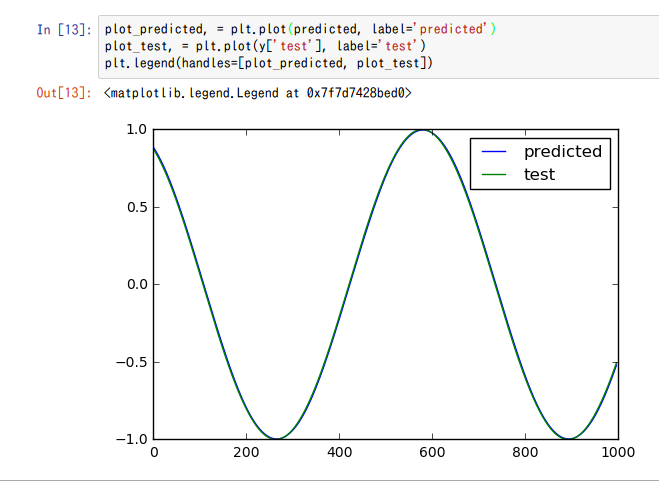
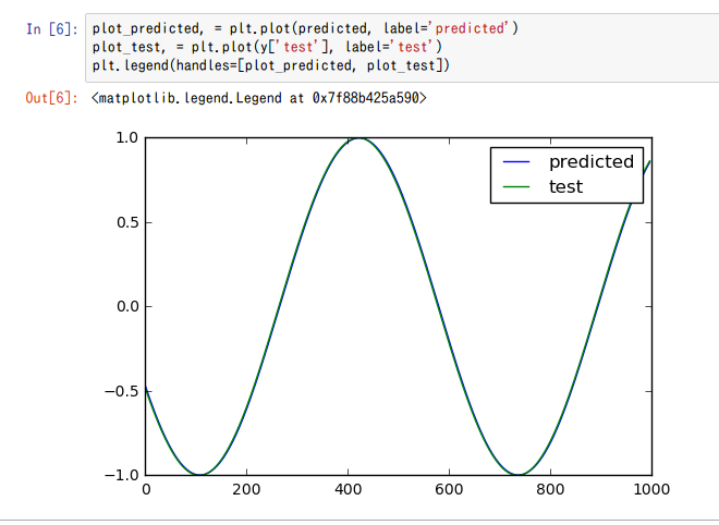
plot_predicted, = plt.plot(predicted, label='predicted')
plot_test, = plt.plot(y['test'], label='test')
plt.legend(handles=[plot_predicted, plot_test])

グラフ描画。

cosineにしてみた

cosine curveとしても位相が0からでないようだが未消化だった。

Xの値

Xにはtrainとtestがあるようだ。

X['train']

array([[[ 1.        ],
        [ 0.99994999],
        [ 0.99979997]],

       [[ 0.99994999],
        [ 0.99979997],
        [ 0.99954993]],
...

testの方は値域が-0.45610371から始まっているようだ。

X['test']

array([[[-0.45610371],
        [-0.46498191],
        [-0.47380689]],

       [[-0.46498191],
        [-0.47380689],
        [-0.48259121]],

       [[-0.47380689],
        [-0.48259121],
        [-0.49132726]],

       ..., 
       [[ 0.83593178],
        [ 0.8413794 ],
        [ 0.84673876]],

       [[ 0.8413794 ],
        [ 0.84673876],
        [ 0.85201752]],

       [[ 0.84673876],
        [ 0.85201752],
        [ 0.85721111]]], dtype=float32)

X.keys

['test', 'train', 'val']

len(X['train'])

len(X['test'])

len(X['val'])

この３つの値をどこで設定しているかは未消化だった。
8097 + 997 + 897 = 9991.

リンク記事でだいたい解決した。
http://qiita.com/7of9/items/d970baf3322b93efb02b