TensorFlow APIメモ

TensorFlowのAPI

TensorFlowのAPIについて調べたことをメモしていきます。調べていく度に追加していきます。
バージョン1.21で確認しています。

参考リンク

• TensorFlowをWindowsにインストール Python初心者でも簡単だった件
• 【入門者向け解説】TensorFlow基本構文とコンセプト
• 【入門者向け解説】TensorFlowチュートリアルMNIST(初心者向け)
• 【TensorBoard入門】TensorFlow処理を見える化して理解を深める
• 【TensorBoard入門:image編】TensorFlow画像処理を見える化して理解を深める
• 【TensorBoard入門:Projector編】TensorFlow処理をかっこよく見える化
• TensorFlowチュートリアルMNIST(初心者向け)をTensorBoardで見える化
• 【入門者向け解説】TensorFlowチュートリアルDeep MNIST
• Jupyter Notebookでmatplotlibをインストールしてグラフ表示
• TensorFlow理解のために柏木由紀さん顔特徴を調べてみた【前編】

shape

説明

Tensorの次元の要素数を返してくれます。画像ファイルのサイズはこれで見ました。

基本構文

shape(
    input,
    name=None,
    out_type=tf.int32
)

例1

1次元の3要素配列のshapeを返す

import tensorflow as tf
sess = tf.InteractiveSession()
print(sess.run(tf.shape((tf.range(3)))))

結果

[3]

例2

0から11までをReshapeしてTensorに格納。そのShapeを返す。

import tensorflow as tf
sess = tf.InteractiveSession()
three_dim = tf.reshape(tf.range(6),[1,2,3])
print(sess.run(three_dim))
print(sess.run(tf.shape(three_dim)))

結果(上がTensor内容で、下がshape結果)

[[[0 1 2]
[3 4 5]]]

[1 2 3]

range

説明

数値を順番に作ってくれます。動作確認時に重宝します。

基本構文

range(limit, delta=1, dtype=None, name='range')
range(start, limit, delta=1, dtype=None, name='range'))

例1

0から11までをTensorに格納

import tensorflow as tf
sess = tf.InteractiveSession()
print(sess.run(tf.range(12)))

結果

[ 0 1 2 3 4 5 6 7 8 9 10 11]

例2

0から11までをReshapeしてTensorに格納。動作確認としては、この方法が重宝します。

import tensorflow as tf
sess = tf.InteractiveSession()
print(sess.run(tf.reshape(tf.range(12), [3,4])))

結果

[[ 0 1 2 3]
[ 4 5 6 7]
[ 8 9 10 11]]

reshape

説明

テンソルの形式を変換。

基本構文

reshape(
    tensor,
    shape,
    name=None
)

例1

0から11までの1次元配列を2×6の2次元配列に変換

import tensorflow as tf
sess = tf.InteractiveSession()
print(sess.run(tf.reshape(tf.range(12), [2,6])))

結果

[[ 0 1 2 3 4 5]
[ 6 7 8 9 10 11]]

例2

0から11までの1次元配列を2×3×2の3次元配列に変換

import tensorflow as tf
sess = tf.InteractiveSession()
print(sess.run(tf.reshape(tf.range(12), [2,3,2])))

結果

[[[ 0 1]
[ 2 3]
[ 4 5]]

[[ 6 7]
[ 8 9]
[10 11]]]

例3

0から11までの1次元配列を2×3×2の3次元配列に変換(-1を使用)
-1はワイルドカードの意味で1回だけ使えます([-1,-1,2]みたいな使い方はだめ)。
今回の例だと12の変数を$12 ÷ 2 ÷ 2 = 3$として3を計算してくれます。

import tensorflow as tf
sess = tf.InteractiveSession()
print(sess.run(tf.reshape(tf.range(12), [2,-1,2])))

結果

[[[ 0 1]
[ 2 3]
[ 4 5]]

[[ 6 7]
[ 8 9]
[10 11]]]

transpose

説明

テンソルの順序を変換。[TensorFlow] APIドキュメントを眺める -Math編-にわかりやすくのっています。

基本構文

transpose(
    a,
    perm=None,
    name='transpose'
)

例1

0から11までの2×6の2次元配列を順列変換。2次元なので単純な行列変換。

import tensorflow as tf
sess = tf.InteractiveSession()

x = (tf.reshape(tf.range(12), [-1,2]))

print(sess.run(x))
print(sess.run(tf.transpose(x)))

結果

$x$のTensor

[[ 0 1]
[ 2 3]
[ 4 5]
[ 6 7]
[ 8 9]
[10 11]]

$x$をtransposeした結果

[[ 0 2 4 6 8 10]
[ 1 3 5 7 9 11]]

例2

0から11までの4次元配列の順序変換。permで順序指定をしています。今回の例だと元Tensorの3次元目、0次元目、1次元目、2次元目の順に並べ替え。

import tensorflow as tf
sess = tf.InteractiveSession()
y = (tf.reshape(tf.range(12), [2,2,1,3]))

print(sess.run(y))
print(sess.run(tf.transpose(y, perm=[3,0,1,2])))

結果

$y$のTensor

[[[[ 0 1 2]]
[[ 3 4 5]]]
[[[ 6 7 8]]
[[ 9 10 11]]]]

$y$をtransposeした結果

[[[[ 0]
[ 3]]
[[ 6]
[ 9]]]
[[[ 1]
[ 4]]
[[ 7]
[10]]]
[[[ 2]
[ 5]]
[[ 8]
[11]]]]

truncated_normal

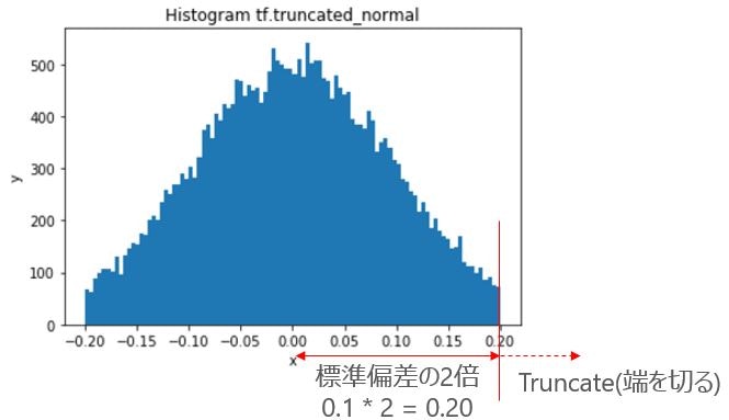
説明

正規分布に従って、標準偏差の2倍までの範囲に限定された乱数を返します。

基本構文

truncated_normal(
    shape,
    mean=0.0,
    stddev=1.0,
    dtype=tf.float32,
    seed=None,
    name=None
)

例

標準偏差0.1の乱数を30000万作成してヒストグラムとして表示。

import tensorflow as tf
import numpy as np
import matplotlib.pyplot as plt
sess = tf.InteractiveSession()
x = sess.run(tf.truncated_normal([30000], stddev=0.1))
fig = plt.figure()
ax = fig.add_subplot(1,1,1)

ax.hist(x, bins=100)
ax.set_title('Histogram tf.truncated_normal')
ax.set_xlabel('x')
ax.set_ylabel('y')
plt.show()

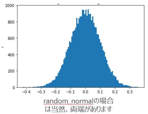
こちらは参考(random_normalで、通常の正規分布)

tf.app.run

説明

関数のラッパ。引数mainがNoneの場合 main.main が実行される。コマンドで呼び出す時に便利っぽい。英語ですがStackoverflowに詳しく載っています。

基本構文

run(
    main=None,
    argv=None
)

tf.summary.scalar

説明

TensorBoardのグラフに出力する。

基本構文

scalar(
    name,
    tensor,
    collections=None
)

例

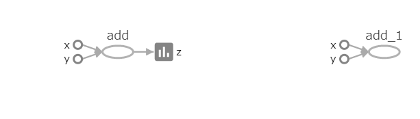
$x+y$の値をTensorBoardに出力。tf.summary.scalarの使用有無で比較

import tensorflow as tf
sess = tf.InteractiveSession()

# TensorBoard情報出力ディレクトリ
log_dir = '/tmp/tensorflow/mnist/logs/try01'

# 指定したディレクトリがあれば削除し、再作成
if tf.gfile.Exists(log_dir):
    tf.gfile.DeleteRecursively(log_dir)
tf.gfile.MakeDirs(log_dir)

# 定数で1 + 2
x = tf.constant(1, name='x')
y = tf.constant(2, name='y')
z_out    = x + y
z_no_out = x + y

# このコマンドでzをグラフ上に出力
tf.summary.scalar('z', z_out)

# SummaryWriterでグラフを書く
summary_writer = tf.summary.FileWriter(log_dir , sess.graph)

# 実行
print(sess.run(z_out))
print(sess.run(z_no_out))

# SummaryWriterクローズ
summary_writer.close()

結果(左がtf.summary.scalarを使った場合で、右が使わなかった場合)