【TensorBoard入門:image編】TensorFlow画像処理を見える化して理解を深める

TensorBoardでTensorFlowの理解を早める

TensorFlowの畳み込み処理・プーリング処理の過程を確認したく、TensorBoardに出力しました。その時の画像確認方法のメモです。前提として、基本的な使い方は「【TensorBoard入門】TensorFlow処理を見える化して理解を深める」を参照ください。
環境:python3.5 tensorflow1.21

参考リンク

• TensorFlowをWindowsにインストール Python初心者でも簡単だった件
• 【入門者向け解説】TensorFlow基本構文とコンセプト
• 【入門者向け解説】TensorFlowチュートリアルMNIST(初心者向け)
• 【TensorBoard入門】TensorFlow処理を見える化して理解を深める
• 【TensorBoard入門:Projector編】TensorFlow処理をかっこよく見える化
• TensorFlowチュートリアルMNIST(初心者向け)をTensorBoardで見える化
• 【入門者向け解説】TensorFlowチュートリアルDeep MNIST
• TensorFlow APIメモ
• TensorFlow理解のために柏木由紀さん顔特徴を調べてみた【前編】

TensorBoard(Image)の簡単なロジック

手書き数値文字(MNIST)を見る

ただ手書き数値文字(MNIST)を見るだけのコードを書いてみます。

import tensorflow as tf
sess = tf.InteractiveSession()
# MNISTデータ読込
from tensorflow.examples.tutorials.mnist import input_data
mnist = input_data.read_data_sets('MNIST_data', one_hot=True)

# TensorBoard情報出力ディレクトリ
log_dir = '/tmp/tensorflow/test/tensorboard_image01'

# 指定したディレクトリがあれば削除し、再作成
if tf.gfile.Exists(log_dir):
    tf.gfile.DeleteRecursively(log_dir)
tf.gfile.MakeDirs(log_dir)

# 画像データを入れるPlaceholder
x  = tf.placeholder(tf.float32, shape=[None, 784])

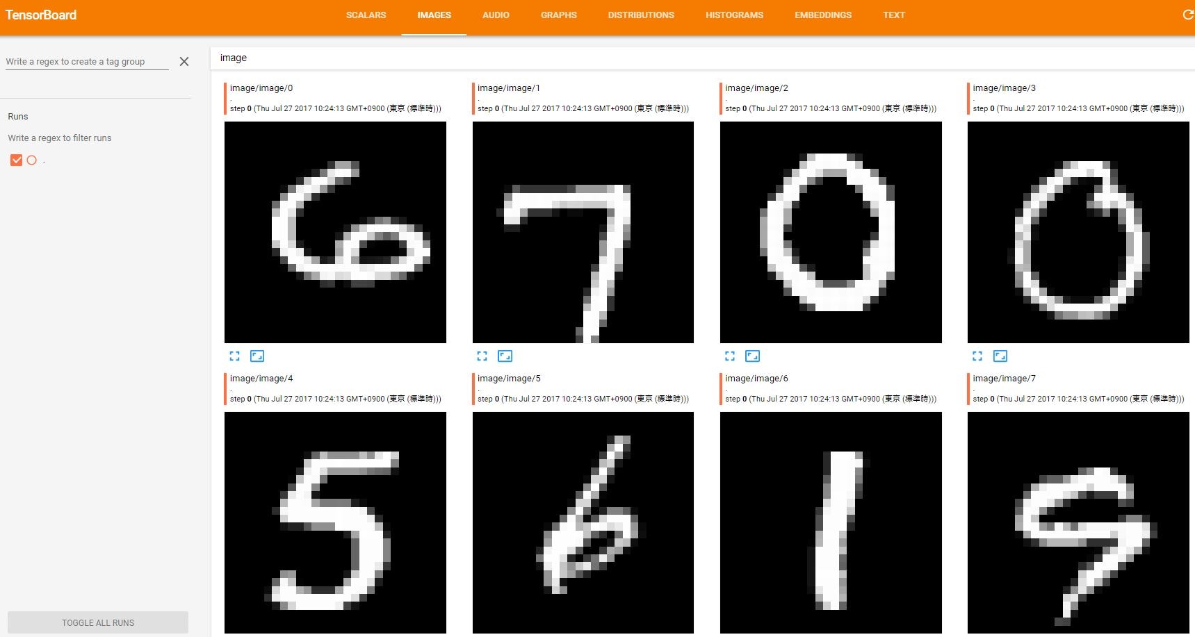
# 画像を28×28に変換してTensorboardに10件出力
_ = tf.summary.image('image', tf.reshape(x, [-1, 28, 28, 1]), 10)
merged = tf.summary.merge_all()

# minst画像の取得
batch = mnist.train.next_batch(10)

# 実行
summary = sess.run(merged, feed_dict={x: batch[0]})

# Writer処理
summary_writer = tf.summary.FileWriter(log_dir, sess.graph)
summary_writer.add_summary(summary)
summary_writer.close()

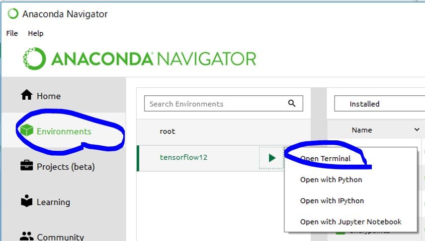
その後にTensorboardを起動します。筆者の環境はAnacondaで構築しているので、まずAnaconda NavigatorからTerminalを起動しています。

で、TerminalからTensorbaordをディレクトリを指定して起動します(Pythonプログラム内変数log_dirにディレクトリを格納しています)。

tensorboard --logdir=/tmp/tensorflow/mnist/logs/simple01

起動後にブラウザで http://localhost:6006/ を開くとTensorBoard画面が表示されます。

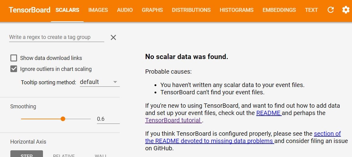
「No scalar data was found(データがないぞ)」と怒られますが、今回はscalarは出力しておらず、Graph出力のみとしているので問題ありません。画面上にあるメニューで「Images」を選ぶことで画像を見ることができます。

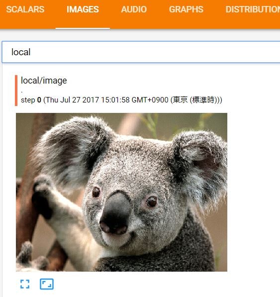
ローカルファイルの画像を見る

説明

ローカルファイルを読み込んで出力します。ローカルファイル読込方法に関しては、記事「オリジナルのデータセットを読み込むための準備」を参考にしました。

import tensorflow as tf
sess = tf.InteractiveSession()

# TensorBoard情報出力ディレクトリ
log_dir = '/tmp/tensorflow/test/tensorboard_image02'

# 指定したディレクトリがあれば削除し、再作成
if tf.gfile.Exists(log_dir):
    tf.gfile.DeleteRecursively(log_dir)
tf.gfile.MakeDirs(log_dir)

# ファイル場所("C:\\"部分はエスケープ処理のため、"\"が2つあることに注意)
jpg = tf.read_file('C:\\Users\yohei.fukuhara\Pictures\Saved Pictures\Sample Pictures\Koala.jpg')

# JPEGファイルデコード(tf.image.decode_pngや万能なtf.image.decode_imageもあり)
img_raw = tf.image.decode_jpeg(jpg, channels=3)

# 画像サイズを取得(画像ファイルプロパティからも確認可能)
img_shape = tf.shape(img_raw)

# 画像をTensorboardに出力
_ = tf.summary.image('local', tf.reshape(img_raw, [-1, img_shape[0], img_shape[1], img_shape[2]]), 1)
merged = tf.summary.merge_all()

# 実行
summary = sess.run(merged)

# Writer処理
summary_writer = tf.summary.FileWriter(log_dir, sess.graph)
summary_writer.add_summary(summary)
summary_writer.close()

結果が出てきます。

エキスパート向けチュートリアルDeep MNIST for Experts

いよいよ本題です。エキスパート向けチュートリアルで畳み込み処理、プーリング処理の過程を見ていきます。コードは以下のとおりです。

import tensorflow as tf
sess = tf.InteractiveSession()
# MNISTデータ読込
from tensorflow.examples.tutorials.mnist import input_data
mnist = input_data.read_data_sets('MNIST_data', one_hot=True)

# TensorBoard情報出力ディレクトリ
log_dir = '/tmp/tensorflow/mnist/logs/mnist_expert_images'

# 指定したディレクトリがあれば削除し、再作成
if tf.gfile.Exists(log_dir):
    tf.gfile.DeleteRecursively(log_dir)
tf.gfile.MakeDirs(log_dir)

# Input placeholders & 画像変換
with tf.name_scope('input'):
    x  = tf.placeholder(tf.float32, shape=[None, 784], name='x-input')
    y_ = tf.placeholder(tf.float32, shape=[None, 10],  name='y-input')

    # 画像を28×28に変換
    x_image = tf.reshape(x, [-1, 28, 28, 1])
    tf.summary.image('preprocess', x_image, 10)

# 変数を加工してTensorBoard出力する関数
def variable_summaries(var):

    # 変数Summaries
    with tf.name_scope('summaries'):
        mean = tf.reduce_mean(var)                      #Scalar出力(平均)
        tf.summary.scalar('mean', mean)
        with tf.name_scope('stddev'):
            stddev = tf.sqrt(tf.reduce_mean(tf.square(var - mean)))
        tf.summary.scalar('stddev', stddev)             #Scalar出力(標準偏差)
        tf.summary.scalar('max', tf.reduce_max(var))    #Scalar出力(最大値)
        tf.summary.scalar('min', tf.reduce_min(var))    #Scalar出力(最小値)
        tf.summary.histogram('histogram', var)          #ヒストグラム出力

# 重み付け値
def weight_variable(shape):
    initial = tf.truncated_normal(shape, stddev=0.1)    #標準偏差0.1の正規分布乱数
    return tf.Variable(initial)

# バイアス値
def bias_variable(shape):
    initial = tf.constant(0.1, shape=shape)             #初期値0.1定数
    return tf.Variable(initial)

# 畳み込み処理
def conv2d(x, W):
    return tf.nn.conv2d(x, W, strides=[1, 1, 1, 1], padding='SAME')

# Max Pooling
def max_pool_2x2(x):
    return tf.nn.max_pool(x, ksize=[1, 2, 2, 1], strides=[1, 2, 2, 1], padding='SAME')

# 第1層
with tf.name_scope('1st_layer'):

    # 第1畳み込み層
    with tf.name_scope('conv1_layer'):
        with tf.name_scope('weight'):
            W_conv1 = weight_variable([5, 5, 1, 32])
            variable_summaries(W_conv1)

            #Tensorを[5,5,1,32]から[32,5,5,1]と順列変換してimage出力
            tf.summary.image('filter', tf.transpose(W_conv1,perm=[3,0,1,2]), 10)

        with tf.name_scope('bias'):            
            b_conv1 = bias_variable([32])
            variable_summaries(b_conv1)
        with tf.name_scope('activations'):            
            h_conv1 = tf.nn.relu(conv2d(x_image, W_conv1) + b_conv1)
            tf.summary.histogram('activations', h_conv1)

            #Tensorを[-1,28,28,32]から[-1,32,28,28]と順列変換し、[-1]と[-32]をマージしてimage出力
            tf.summary.image('convolved', tf.reshape(tf.transpose(h_conv1,perm=[0,3,1,2]),[-1,28,28,1]), 10)

# 第1プーリング層
    with tf.name_scope('pool1_layer'):    
        h_pool1 = max_pool_2x2(h_conv1)

        #Tensorを[-1,14,14,32]から[-1,32,14,14]と順列変換し、[-1]と[32]をマージしてimage出力
        tf.summary.image('pooled', tf.reshape(tf.transpose(h_pool1,perm=[0,3,1,2]),[-1,14,14,1]), 10)

#第2層
with tf.name_scope('2nd_layer'):

    # 第2畳み込み層
    with tf.name_scope('conv2_layer'):
        with tf.name_scope('weight'):
            W_conv2 = weight_variable([5, 5, 32, 64])
            variable_summaries(W_conv2)

            #Tensorを[5,5,32,64]から[32*64,5,5,1]と順列変換してimage出力
            tf.summary.image('filter', tf.reshape(tf.transpose(W_conv2,perm=[2,3,0,1]),[-1,5,5,1]), 20)
        with tf.name_scope('bias'):            
            b_conv2 = bias_variable([64])
            variable_summaries(b_conv2)
        with tf.name_scope('activations'):
            h_conv2 = tf.nn.relu(conv2d(h_pool1, W_conv2) + b_conv2)
            tf.summary.histogram('activations', h_conv2)
            #Tensorを[-1,14,14,64]から[-1,64,14,14]と順列変換し、[-1]と[64]をマージしてimage出力
            tf.summary.image('convolved', tf.reshape(tf.transpose(h_conv2,perm=[0,3,1,2]),[-1,14,14,1]), 10)

# 第2プーリング層
    with tf.name_scope('pool2_layer'):
        h_pool2 = max_pool_2x2(h_conv2)

        #Tensorを[-1,7,7,64]から[-1,64,7,7]と順列変換し、[-1]と[64]をマージしてimage出力
        tf.summary.image('pooled', tf.reshape(tf.transpose(h_pool2,perm=[0,3,1,2]),[-1,7,7,1]), 10)

# 密結合層
with tf.name_scope('fc1_layer'):
    h_pool2_flat = tf.reshape(h_pool2, [-1, 7*7*64])
    with tf.name_scope('weight'):
        W_fc1 = weight_variable([7 * 7 * 64, 1024])
        variable_summaries(W_fc1)
    with tf.name_scope('bias'):            
        b_fc1 = bias_variable([1024])
        variable_summaries(b_fc1)
    with tf.name_scope('activations'):
        h_fc1 = tf.nn.relu(tf.matmul(h_pool2_flat, W_fc1) + b_fc1)
        tf.summary.histogram('activations', h_fc1)

    #ドロップアウト
    with tf.name_scope('dropout'):
        keep_prob  = tf.placeholder(tf.float32)
        tf.summary.scalar('dropout_keep_probability', keep_prob)
        h_fc1_drop = tf.nn.dropout(h_fc1, keep_prob)

# 読み出し層
with tf.name_scope('fc2_layer'):
    with tf.name_scope('weight'):
        W_fc2 = weight_variable([1024, 10])
        variable_summaries(W_fc2)
    with tf.name_scope('bias'):            
        b_fc2 = bias_variable([10])
        variable_summaries(b_fc2)
    with tf.name_scope('preactivations'):
        y_conv = tf.matmul(h_fc1_drop, W_fc2) + b_fc2
        tf.summary.histogram('preactivations', y_conv)

# 交差エントロピー(クロスエントロピー)算出
with tf.name_scope('cross_entropy'):
    cross_entropy = tf.reduce_mean(tf.nn.softmax_cross_entropy_with_logits(labels=y_, logits=y_conv))
    tf.summary.scalar("cross_entropy", cross_entropy)

# 訓練
with tf.name_scope('train'):
    train_step = tf.train.AdamOptimizer(1e-4).minimize(cross_entropy)

# 正答率計算
with tf.name_scope('accuracy'):
    correct_prediction = tf.equal(tf.argmax(y_conv, 1), tf.argmax(y_, 1))
    accuracy = tf.reduce_mean(tf.cast(correct_prediction, tf.float32))
    tf.summary.scalar('accuracy', accuracy)

# 全Summariesを出力
merged = tf.summary.merge_all()
train_writer = tf.summary.FileWriter(log_dir + '/train', sess.graph) #訓練データ
test_writer  = tf.summary.FileWriter(log_dir + '/test')              #テストデータ

# 初期化
tf.global_variables_initializer().run()

# 訓練・テスト繰り返し    
for i in range(3000):
    batch = mnist.train.next_batch(50)

    #100回ごとに訓練トレース詳細
    if i % 100 == 0:
        run_options  = tf.RunOptions(trace_level=tf.RunOptions.FULL_TRACE)
        run_metadata = tf.RunMetadata()
        summary, train_accuracy, _   = sess.run([merged, accuracy , train_step],
                                                feed_dict={x: batch[0], y_:batch[1], keep_prob: 1.0},
                                                options=run_options,
                                                run_metadata=run_metadata)
        train_writer.add_run_metadata(run_metadata, 'step%03d' % i)
        train_writer.add_summary(summary, i)
        print('step %d, training accuracy %g' % (i, train_accuracy))
    #100回ごとにテスト
    elif i % 100 == 99:
        summary_test, train_accuracy = sess.run([merged, accuracy], feed_dict={x: mnist.test.images, y_:mnist.test.labels, keep_prob: 1.0})
        test_writer.add_summary(summary_test, i)

    #訓練結果書き込み
    summary, _ = sess.run([merged, train_step], feed_dict={x: batch[0], y_: batch[1], keep_prob: 0.5})
    train_writer.add_summary(summary, i)

#最終テスト結果出力
print('test accuracy %g' % accuracy.eval(feed_dict={x: mnist.test.images, y_: mnist.test.labels, keep_prob: 1.0}))

# Writerクローズ
train_writer.close()
test_writer.close()

結果
名称(input, 1st_layer, 2nd_layer)ごとにグルーピングされています。記事「【入門者向け解説】TensorFlowチュートリアルDeep MNIST」も参照ください。

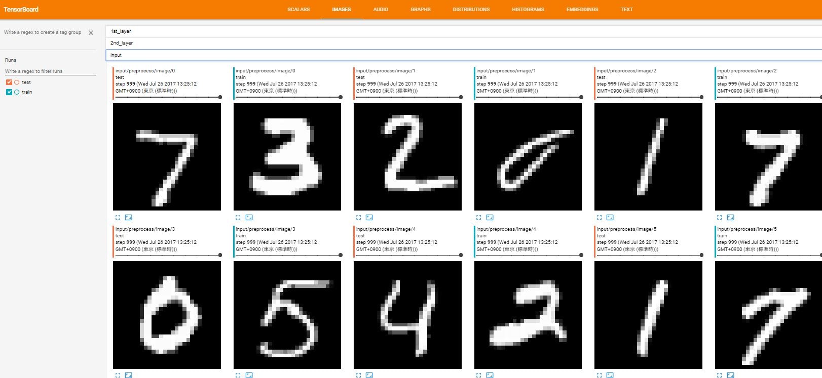
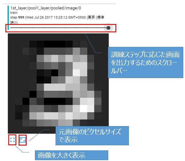
訓練ステップに応じて画像出力できるのがいいです。