
Pipelineを使いたいけど、痒いところに手が届かない
Scikit-learnのPipelineを使うと前処理からモデル構築までを一度呼び出すことができるので処理がとてもすっきりします。GridSearchとも相性が良く、Kaggleのプロジェクトにもよく使います。
パイプが直列に並べられる時は、詰まるところはないですが、「データを分割してそれぞれ別の処理を行いマージさせる」といった並列的な経路の処理や「前処理後の変数名を得たい」のようなパイプ内の情報を得たい時には、適宜やり方を調べていたのでこの記事にまとめました!!
💡この記事で紹介すること
- まずは普通にPipelineでモデル作成
- パイプに自作の関数を組み込む(FunctionTransformer)
- パイプを分岐させる(ColumnTransformer)
- パイプ内でつくった色々なデータを取得する
Pipelineの構築
まずは普通に使ってモデル作成
KaggleのSpaceship Titanicを題材にします。Pipelineを使ったことがある方は飛ばしても大丈夫です。
このコンペは乗客が異次元に転送されたかどうかを推論する2値分類問題です。
説明変数は13個で、6個がnumerical、7個がcategoricalです。
[in]
import pandas as pd
df = pd.read_csv('/kaggle/input/spaceship-titanic/train.csv')
df.dtypes

[out]
PassengerId      object
HomePlanet       object
CryoSleep        object
Cabin            object
Destination      object
Age             float64
VIP              object
RoomService     float64
FoodCourt       float64
ShoppingMall    float64
Spa             float64
VRDeck          float64
Name             object
Transported        bool
dtype: object
早速、Pipelineを組んでいきます。
欠損値があるので、imputerを使います。
[in]
# 各列の欠損値の数を確認
df.isnull().sum()

[out]
PassengerId       0
HomePlanet      201
CryoSleep       217
Cabin           199
Destination     182
Age             179
VIP             203
RoomService     181
FoodCourt       183
ShoppingMall    208
Spa             183
VRDeck          188
Name            200
Transported       0
dtype: int64
さらにカテゴリ変数が含まれているのでOne-Hotエンコーディングをします。
モデルとしては決定木分析を採用します。
[in]
import numpy as np
from sklearn.pipeline import Pipeline
from sklearn.model_selection import train_test_split
from sklearn.impute import SimpleImputer
from sklearn.preprocessing import OneHotEncoder
from sklearn.tree import DecisionTreeClassifier

target = 'Transported'
X = df.drop([target], axis=1)
y = df[target]
X_train, X_test, y_train, y_test = train_test_split(X, y, test_size=0.2, random_state=0)

clf = DecisionTreeClassifier(max_depth=4,random_state=1234)

# ここからがPipeline
simple_pipeline = Pipeline(
    steps=[
        ('imputer', SimpleImputer(strategy='most_frequent')),
        ('encoder', OneHotEncoder(handle_unknown='ignore',sparse=False)),
        ('model', clf)
    ],
    verbose=True
)

[out]
出来上がったPipelineはこちらです。

通常のscikit-learnのモデルと同じように扱うことができます。
[in]
simple_pipeline.fit(X_train,y_train)
print('='*30)
print('推論結果:', simple_pipeline.predict(X_test))
print('='*30)
print('trainデータでのスコア:', simple_pipeline.score(X_train, y_train))
print('='*30)
print('testデータでのスコア:', simple_pipeline.score(X_test,y_test))

[out]
[Pipeline] ........... (step 1 of 3) Processing imputer, total=   0.0s
[Pipeline] ........... (step 2 of 3) Processing encoder, total=   0.1s
[Pipeline] ............. (step 3 of 3) Processing model, total=   0.0s
==============================
推論結果: [False  True False ...  True False False]
==============================
trainデータでのスコア: 0.7335346563129135
==============================
testデータでのスコア: 0.721679125934445
パイプに自作の関数を組み込む
まずはモデルをつくってみましたが、不要な変数があるので取り除きます。単純なdrop()メソッドですが、こちらを自作関数としてPipelineに組み込みます。
削除するのはPassengerID、Cabin、Name列です。(Cabinは有用な変数ですが、今回は前処理が面倒なので削除します)
関数を定義します。
def processing1(dataframe):
    return dataframe.drop(['PassengerId','Cabin','Name'], axis=1)
こちらをFunctionTransformer()を使い変換すれば、Pipelineに組み込むことができます。
[in]
from sklearn.preprocessing import FunctionTransformer
# 自作関数を変換
myfunc = FunctionTransformer(processing1)

clf = DecisionTreeClassifier(max_depth=4,random_state=1234)

myfunc_pipeline = Pipeline(
    steps=[
        ('dropcol', myfunc), # ←ここに組み込む
        ('imputer', SimpleImputer(strategy='most_frequent')),
        ('encoder', OneHotEncoder(handle_unknown='ignore',sparse=False)),
        ('model', clf)
    ],
    verbose=True
)
myfunc_pipeline.fit(X_train,y_train)
print('='*30)
print('推論結果:', myfunc_pipeline.predict(X_test))
print('='*30)
print('trainデータでのスコア:', myfunc_pipeline.score(X_train, y_train))
print('='*30)
print('testデータでのスコア:', myfunc_pipeline.score(X_test,y_test))

[out]
[Pipeline] ........... (step 1 of 4) Processing dropcol, total=   0.0s
[Pipeline] ........... (step 2 of 4) Processing imputer, total=   0.0s
[Pipeline] ........... (step 3 of 4) Processing encoder, total=   0.3s
[Pipeline] ............. (step 4 of 4) Processing model, total=   1.6s
==============================
推論結果: [False  True False ...  True False False]
==============================
trainデータでのスコア: 0.7484900776531492
==============================
testデータでのスコア: 0.7372052903967797
パイプを分岐させる
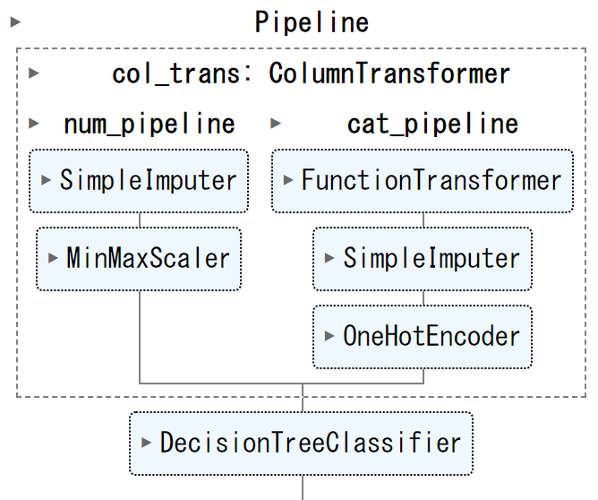
続いて、カテゴリ変数にはOne-Hotエンコーディングをしましたが、連続変数に対しては何もしていないのでMinMax法で正規化します。この時、データ型によって処理内容を変えたいので、Pipelineを分岐させます。
このようなイメージです。
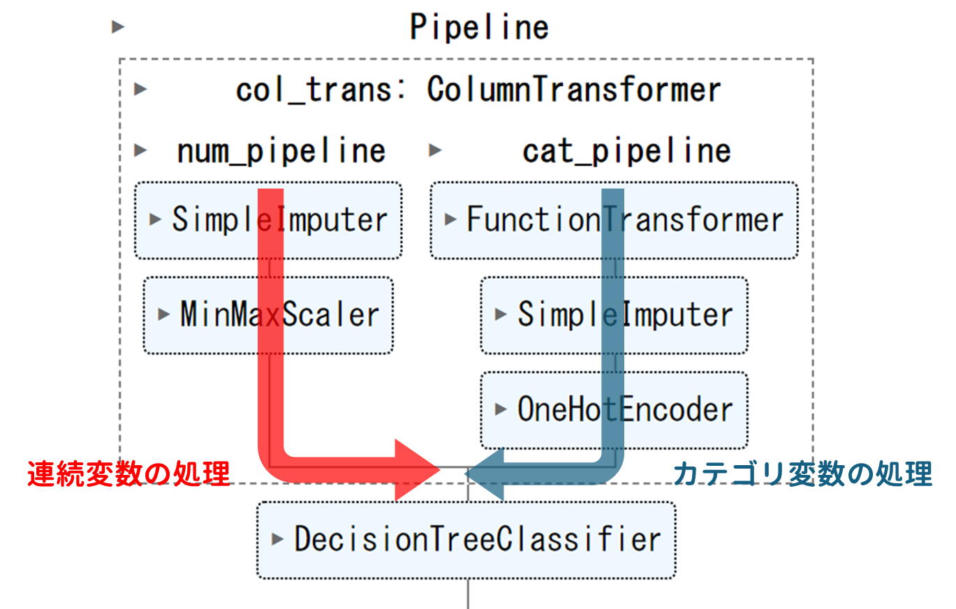
分岐する際はColumnTransformer()を使います。
ソースコードはこちら
from sklearn.compose import ColumnTransformer
from sklearn.preprocessing import OneHotEncoder,MinMaxScaler

# 連続変数の列名を取得
n_cols = df.loc[:,df.dtypes=='float'].columns
# カテゴリ変数の列名を取得
c_cols = df.loc[:,df.dtypes=='object'].columns

# 連続変数のPipeline(図の左側の赤いライン)
num_pipeline = Pipeline(
    steps=[
        ('impute', SimpleImputer(strategy='mean')),
        ('scale',MinMaxScaler())
    ]
)

# カテゴリ変数のPipeline(図の右側の青いライン)
cat_pipeline = Pipeline(
    steps=[
        ('drop', myfunc),
        ('imputer', SimpleImputer(strategy='most_frequent')),
        ('encoder', OneHotEncoder(handle_unknown='ignore',sparse=False))
    ],
    verbose=True
)

# 分岐するPipelineの構築. ここが大事!
ct = ColumnTransformer(
    transformers=[
        ('num_pipeline',num_pipeline,np.array(n_cols)),
        ('cat_pipeline',cat_pipeline,np.array(c_cols))
    ],
remainder='drop',n_jobs=-1)

# 決定木分析のモデルに結合
clf = DecisionTreeClassifier(max_depth=4,random_state=1234)
parallel_pipeline = Pipeline(
    steps=[
        ('col_trans',ct),
        ('model', clf)
    ]
)

parallel_pipeline.fit(X_train,y_train)
print('='*30)
print('推論結果:', parallel_pipeline.predict(X_test))
print('='*30)
print('trainデータでのスコア:', parallel_pipeline.score(X_train, y_train))
print('='*30)
print('testデータでのスコア:', parallel_pipeline.score(X_test,y_test))

[out]
[Pipeline] ......... (step 1 of 2) Processing col_trans, total=   0.1s
[Pipeline] ............. (step 2 of 2) Processing model, total=   0.0s
==============================
推論結果: [ True  True False ...  True False  True]
==============================
trainデータでのスコア: 0.7730802415875755
==============================
testデータでのスコア: 0.7636572742955722
経路のおさらいです。
パイプ内でつくった色々なデータを取得する
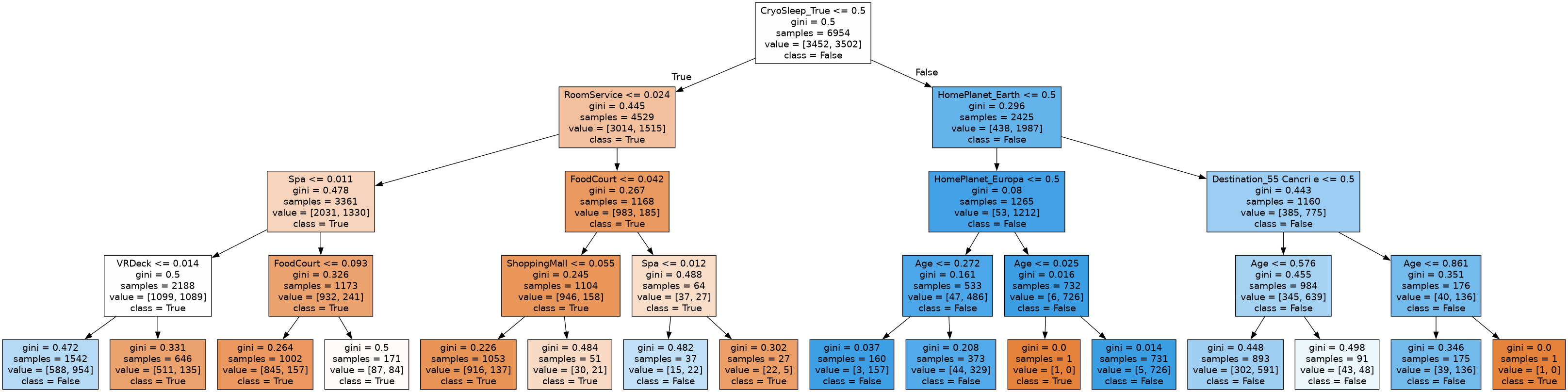
例として、ツリーをgraphvizで描画します。このようなイメージです。

このためにモデルと変数名を取得します。変数名はOne-Hotエンコーディング処理をした後のものを手に入れる必要があります。
図の〇で囲った時点の変数を取得しマージします。
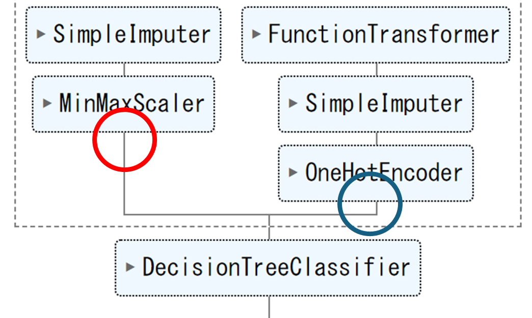
ソースコードはこちら
[in]
# モデルの取得はとても簡単
model = parallel_pipeline['model']

# 連続変数(図の赤丸). 変数名は変わっていないので実際にはdf.dtypes=='float'と同じ
n_cols_new = parallel_pipeline.named_steps['col_trans'].named_transformers_['num_pipeline'].get_feature_names_out()
print('連続変数:')
print(n_cols_new)

# カテゴリ変数(図の青丸)
c_cols_new = parallel_pipeline.named_steps['col_trans'].named_transformers_['cat_pipeline'].named_steps['encoder'].get_feature_names_out()
print('カテゴリ変数:')
print(c_cols_new)

feature_names = list(n_cols_new) + list(c_cols_new)
print('説明変数:')
print(feature_names)

[out]
連続変数:
array(['Age', 'RoomService', 'FoodCourt', 'ShoppingMall', 'Spa', 'VRDeck'],
      dtype=object)
カテゴリ変数:
array(['HomePlanet_Earth', 'HomePlanet_Europa', 'HomePlanet_Mars',
       'CryoSleep_False', 'CryoSleep_True', 'Destination_55 Cancri e',
       'Destination_PSO J318.5-22', 'Destination_TRAPPIST-1e',
       'VIP_False', 'VIP_True'], dtype=object)
説明変数:
['Age',
 'RoomService',
 'FoodCourt',
 'ShoppingMall',
 'Spa',
 'VRDeck',
 'HomePlanet_Earth',
 'HomePlanet_Europa',
 'HomePlanet_Mars',
 'CryoSleep_False',
 'CryoSleep_True',
 'Destination_55 Cancri e',
 'Destination_PSO J318.5-22',
 'Destination_TRAPPIST-1e',
 'VIP_False',
 'VIP_True']
モデルと変数名を使って描画します
from sklearn import tree
import graphviz

dot_data = tree.export_graphviz(model, out_file=None,
                                feature_names=feature_names,
                                class_names=['True','False'],
                                filled=True)

# Draw graph
graph = graphviz.Source(dot_data, format="png")
graph
変数の重要度を描画します。
importances = model.feature_importances_
tree_importances = pd.Series(importances, index=feature_names)

fig, ax = plt.subplots()
tree_importances.plot.bar(ax=ax)
ax.set_title("Feature importances")
fig.tight_layout()
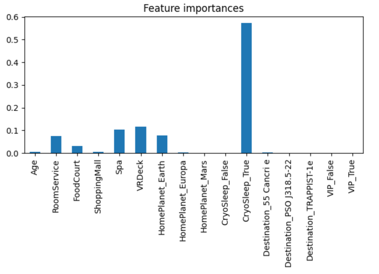
これで実際にモデルの詳細がわかります。
ちなみにPipelineは.fit()や.predict()のようにモデルのようなメソッドを使えますが、そのまま描画に使うことはできません。
[in]
dot_data = tree.export_graphviz(clf_pipeline, out_file=None,
                                feature_names=X_test.columns,
                                class_names=['True','False'],
                                filled=True)
graph = graphviz.Source(dot_data, format="png")
graph

[out]
AttributeError: 'Pipeline' object has no attribute 'tree_'
まとめ
Pipelineは処理が整理できるので、コードの可読性が良くなります。また、今回説明したようなパイプ内のデータの取り出しに慣れるとグラフ作成などの評価も容易になります。
また、この記事では紹介しませんでしたが、このようにGridsearchに組み込むことができます。
from sklearn.pipeline import Pipeline
from sklearn.model_selection import GridSearchCV
gscv = GridSearchCV(PIPELINE, param, cv=10, refit=True, iid=False)