この記事の目的

機械学習モデルを作成する準備段階で、データ内の変数の特徴をとらえたり、注意する点（NaNが多いなど）を洗い出したりするためのメモ．df.info() や df.describe() の拡張版です．

解説

まずはfakerというパッケージを用いてダミーデータを作成します．

!pip install faker

import numpy as np
import pandas as pd
from faker import Faker
import collections

Faker.seed(0)
fake = Faker("ja_JP")

n=1000
df = pd.DataFrame()

for i in range(n):
    df = df.append(fake.profile(), ignore_index=True)

#追加の情報
df["location_lat"] = [d[0] for d in df["current_location"]]
df["location_long"] = [d[1] for d in df["current_location"]]
del df["current_location"], df["website"], df["residence"]
df["income"] = np.random.lognormal(mean=np.log(400), sigma=1/2, size=n)
df["age"] = np.random.randint(low=20, high=100, size=n)

df["birthdate"] = pd.to_datetime(df["birthdate"])
df["member_rank"] = np.random.binomial(n=5, p=0.3, size=n)
df["country"] = ["japan" if np.random.binomial(n=1, p=0.99)==1 else "foreign" for i in range(n)]

#NaNの追加
df["job"] = [d if np.random.binomial(n=1, p=0.95)==1 else np.nan for d in df["job"]]
df["company"] = [d if np.random.binomial(n=1, p=0.9)==1 else np.nan for d in df["company"]]
df["sex"] = [d if np.random.binomial(n=1, p=0.99)==1 else np.nan for d in df["sex"]]
df["blood_group"] = [d if np.random.binomial(n=1, p=0.8)==1 else np.nan for d in df["blood_group"]]
df["mail"] = [d if np.random.binomial(n=1, p=0.05)==1 else np.nan for d in df["mail"]]
df["income"] = [d if np.random.binomial(n=1, p=0.7)==1 else np.nan for d in df["income"]]

df.head()

次に、変数を種類ごとにまとめてデータ型を明示的に指定しておきます．
（例：member_rank にはint型の整数が入っていましたが、順序尺度を想定しているので今回は一旦category型として扱います．LightGBMなどの入力とする際には数値型に戻した方がいいかもしれません．）

########## category ##########
#名義尺度
nominal_list = ["job", "company", "ssn", "blood_group", "username", "name", "sex", "address", "mail", "country"]

#順序尺度
ordinal_list = ["member_rank"]

cate_list = nominal_list+ordinal_list

########## datetime ##########
#日付
date_list = ["birthdate"]

########## number ##########
#間隔尺度
interval_list = ["location_lat", "location_long"]

#比例尺度
ratio_list = ["income", "age"]

num_list = interval_list + ratio_list

for col in cate_list:
    df[col] = df[col].astype("category")

for col in num_list:
    df[col] = df[col].astype("float")

ここから変数の特徴を確認するためのコードです．

def make_bar(num, max_len=20):
    # 0 < num < 1
    num *= max_len
    nan_len = int(np.floor(num)) if num>(max_len/2) else int(np.ceil(num))
    return "".join(["-"]*(max_len-nan_len))+"".join(["|"]*(nan_len))

def get_entropy(arr):
    vs = [v for k,v in collections.Counter(arr).items()]
    ps = vs/np.sum(vs)
    return -np.inner(ps, np.nan_to_num(np.log(ps)))

def make_boxplot(arr, max_len=20):
    q0 = arr.min()
    q1 = arr.quantile(0.25)
    q2 = arr.quantile(0.5)
    q3 = arr.quantile(0.75)
    q4 = arr.max()

    d0 = 0
    d1 = int(np.round((q1-q0)/(q4-q0)*max_len))-1
    d2 = int(np.round((q2-q0)/(q4-q0)*max_len))-1
    d3 = int(np.round((q3-q0)/(q4-q0)*max_len))-1
    d4 = max_len-1

    tmp = ["-"]*20
    tmp[d1] = "|"
    tmp[d2] = "*"
    tmp[d3] = "|"
    return "".join(tmp)

def check_df(df, dtype="category"):
    n = df.shape[0]
    tmp = pd.DataFrame(df.dtypes, columns=["d_type"])
    tmp["nan_count"] = df.isnull().sum(axis=0)
    tmp["nan_vis"] = [make_bar(d/n) for d in tmp["nan_count"]]

    if dtype=="category":
        tmp["n_unique"]=df.nunique()
        tmp["avg_freq(%)"] = (n-tmp["nan_count"])/ n /tmp["n_unique"]*100
        high_freq_list = []
        for i,af in enumerate(tmp["avg_freq(%)"]):
            c = collections.Counter(df.iloc[:,i])
            if np.nan in c:
                del c[np.nan]
            high_freq = c.most_common(1)
            v = c.most_common(1)[0][1] / n*100
            if v > af+10:
                high_freq_list.append(high_freq)
            else:
                high_freq_list.append("")
        tmp["high_freq"] = high_freq_list
        tmp["avg_freq(%)"] = np.round(tmp["avg_freq(%)"],3)
        tmp["entropy"] = [np.round(get_entropy(df.iloc[:,i]),3) for i in range(df.shape[1])]

    elif dtype=="number":
        tmp["mean"] = [np.round(np.nanmean(df.iloc[:,i]),3) for i in range(df.shape[1])]
        tmp["std"] = [np.round(np.nanstd(df.iloc[:,i]),3) for i in range(df.shape[1])]
        tmp["min"] = [np.round(np.nanmin(df.iloc[:,i]),3) for i in range(df.shape[1])]
        tmp["q25"] = [np.round(np.quantile(df.iloc[:,i], q=0.25),3) for i in range(df.shape[1])]
        tmp["median"] = [np.round(np.nanmedian(df.iloc[:,i]),3) for i in range(df.shape[1])]
        tmp["q75"] = [np.round(np.quantile(df.iloc[:,i], q=0.75),3) for i in range(df.shape[1])]
        tmp["max"] = [np.round(np.nanmax(df.iloc[:,i]),3) for i in range(df.shape[1])]
        tmp["boxplot"] = [make_boxplot(df.iloc[:,i]) for i in range(df.shape[1])]
    return tmp

以上までが準備で、以下のように使います．
カテゴリ型の変数のみを指定してdtype="category" として、

check_df(df.loc[:,cate_list], dtype="category")

上の表を見ると、mail のNaNが非常に多かったり、country のほとんどがjapan になっているなど、このまま機械学習モデルの入力として良いのか確認する必要があることが一目でわかります．

数値型の変数のみを指定してdtype="number" として、

check_df(df.loc[:,num_list], dtype="number")

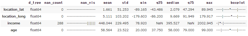
変数 income にはNaNが多少あり、また分布の裾が右に長いことが分かります．

各項目は以下の通りです．

d_type：データ型
nan_count：NaNの件数
nan_vis：NaNの件数を可視化したもの
n_unique：ユニークな要素の数
avg_freq(%)：ユニークな要素１件あたり、データ件数のうち何％を平均的に占めているか
high_freq：最頻値がavg_freq(%)よりも+10%以上占めている場合、高頻度と考えて表示
entropy：多項分布を仮定した下での、データのばらつき度合を表す
mean：平均値
std：標準偏差
min：最小値
q25：25%分位点
median：中央値
q75：75%分位点
max：最大値
boxplot：簡易的にboxplotを表示

参考

PyPI：Faker 6.5.0

特徴量の整理メモ

この記事の目的

解説

参考