概要

ポアソン分布の平均$\lambda$が大きくなると正規分布に近似できるが、その近づく様子を2つの分布の差を取り可視化してみました。可視化してわかる世界をお楽しみください。
ポアソン分布は

P(k)={\frac  {\lambda ^{k}e^{{-\lambda }}}{k!}}

と表される。一方、正規分布は

{\displaystyle f(x)={\frac {1}{\sqrt {2\pi \sigma ^{2}}}}\exp \!\left(-{\frac {(x-\mu )^{2}}{2\sigma ^{2}}}\right)}

と表される。ポアソン分布の$\lambda$が十分に大きいとき、平均$\mu=\lambda$、分散$\sigma ^2=\lambda$の正規分布に近似できる。

実装

Google Colabで作成した本記事のコードは、こちらにあります。

各種インポート

# 各種インポート
import numpy as np
import matplotlib.pyplot as plt
import matplotlib.cm as cm
from scipy.stats import poisson
from scipy.stats import norm
import glob2
import PIL
import IPython  # Google Colabを使う方向け(GIF動画をインライン表示用)

実行時の各種バージョン

Name	Version
numpy	1.21.6
matplotlib	3.2.2
scipy	1.7.3
glob2	0.7
PIL	7.1.2
IPython	5.5.0

ポアソン分布と正規分布の比較

$\lambda$を変えたときの2つの分布を重ねてプロットする。
(コード内では、変数にlambdaは予約語で使えないため、lambda_という変数を使っている。)

lambda_=10

$\lambda=10$のポアソン分布と$\mu=10, \sigma=\sqrt{10}$の正規分布のプロット結果である。(コード内では、変数にlambdaは予約語で使えないため、lambda_という変数を使っている。)

# パラメータ
lambda_ = 10
sigma = np.sqrt(lambda_)
ks = np.arange(0, 30, 1)

# ポアソン分布、正規分布、ポアソン分布 - 正規分布の計算
poisson_distribution = poisson.pmf(ks, lambda_)
normal_distribution = norm.pdf(ks, loc=lambda_, scale=sigma)
diffs = poisson_distribution - normal_distribution

"""図に表示"""
fig, (ax1, ax2) = plt.subplots(figsize=(7, 12), nrows=2, sharex=True)

# ポアソン分布と正規分布のプロット
ax1.plot(ks, poisson_distribution, 'o-', c='red', label='poisson distribution')
ax1.plot(ks, normal_distribution, 'o-', c='blue', label='normal distribution')
ax1.set_ylabel('P(k)')
ax1.legend(loc='upper right')

# ポアソン分布 - 正規分布のプロット
ax2.plot(ks, diffs, label='poisson distribution - normal distribution')
ax2.axhline(0, c="black", ls="--", lw=1, label='0')
ax2.axvline(lambda_, c="black", ls="-", lw=1, label=f'$\lambda$={lambda_}')
ax2.scatter(ks[diffs > 0], diffs[diffs > 0], c='red', label='poisson bigger')
ax2.scatter(ks[diffs < 0], diffs[diffs < 0], c='blue', label='poisson smaller')
ax2.set_ylim(-0.01, 0.01)
ax2.set_xlabel('k')
ax2.set_ylabel(' P_normal(k) - P_poisson(k)')
ax2.legend(loc='upper right')

plt.show()

出力結果

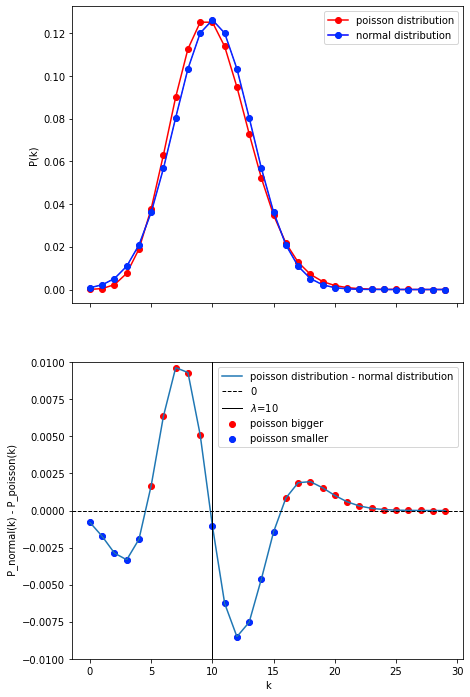
丁度、$\lambda=10$を境に大きくポアソン分布とガウス分布の差が変化していることが分かる。

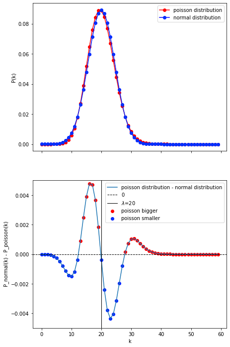
lambda_=20

"""lambda_ = 20"""
# パラメータ
lambda_ = 20
sigma = np.sqrt(lambda_)
ks = np.arange(0, 60, 1)

# ポアソン分布、正規分布、ポアソン分布 - 正規分布の計算
poisson_distribution = poisson.pmf(ks, lambda_)
normal_distribution = norm.pdf(ks, loc=lambda_, scale=sigma)
diffs = poisson_distribution - normal_distribution

"""図に表示"""
fig, (ax1, ax2) = plt.subplots(figsize=(7, 12), nrows=2, sharex=True)

# ポアソン分布と正規分布のプロット
ax1.plot(ks, poisson_distribution, 'o-', c='red', label='poisson distribution')
ax1.plot(ks, normal_distribution, 'o-', c='blue', label='normal distribution')
ax1.set_ylabel('P(k)')
ax1.legend(loc='upper right')

# ポアソン分布 - 正規分布のプロット
ax2.plot(ks, diffs, label='poisson distribution - normal distribution')
ax2.axhline(0, c="black", ls="--", lw=1, label='0')
ax2.axvline(lambda_, c="black", ls="-", lw=1, label=f'$\lambda$={lambda_}')
ax2.scatter(ks[diffs > 0], diffs[diffs > 0], c='red', label='poisson bigger')
ax2.scatter(ks[diffs < 0], diffs[diffs < 0], c='blue', label='poisson smaller')
ax2.set_ylim(-0.005, 0.005)
ax2.set_xlabel('k')
ax2.set_ylabel(' P_normal(k) - P_poisson(k)')
ax2.legend(loc='upper right')

plt.show()

出力結果

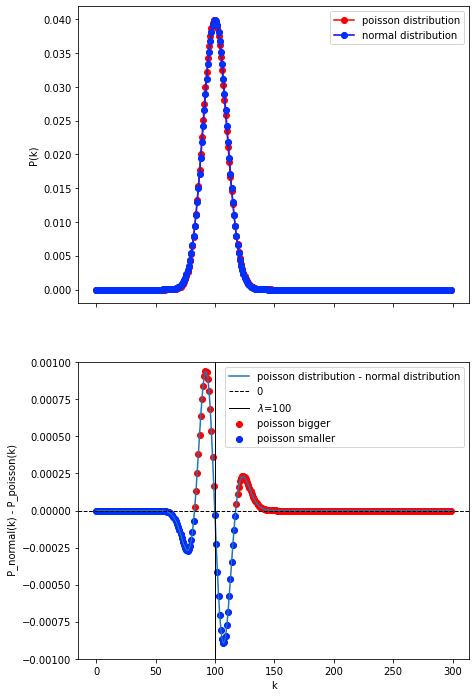
lambda_=100

"""lambda_ = 100"""
# パラメータ
lambda_ = 100
sigma = np.sqrt(lambda_)
ks = np.arange(0, 300, 1)

# ポアソン分布、正規分布、ポアソン分布 - 正規分布の計算
poisson_distribution = poisson.pmf(ks, lambda_)
normal_distribution = norm.pdf(ks, loc=lambda_, scale=sigma)
diffs = poisson_distribution - normal_distribution

"""図に表示"""
fig, (ax1, ax2) = plt.subplots(figsize=(7, 12), nrows=2, sharex=True)

# ポアソン分布と正規分布のプロット
ax1.plot(ks, poisson_distribution, 'o-', c='red', label='poisson distribution')
ax1.plot(ks, normal_distribution, 'o-', c='blue', label='normal distribution')
ax1.set_ylabel('P(k)')
ax1.legend(loc='upper right')

# ポアソン分布 - 正規分布のプロット
ax2.plot(ks, diffs, label='poisson distribution - normal distribution')
ax2.axhline(0, c="black", ls="--", lw=1, label='0')
ax2.axvline(lambda_, c="black", ls="-", lw=1, label=f'$\lambda$={lambda_}')
ax2.scatter(ks[diffs > 0], diffs[diffs > 0], c='red', label='poisson bigger')
ax2.scatter(ks[diffs < 0], diffs[diffs < 0], c='blue', label='poisson smaller')
ax2.set_ylim(-0.001, 0.001)
ax2.set_xlabel('k')
ax2.set_ylabel(' P_normal(k) - P_poisson(k)')
ax2.legend(loc='upper right')

plt.show()

出力結果

考えられる性質

ポアソン分布と正規分布の差は$\sqrt{\lambda}$に反比例するという性質があると考えられる。そこで、$\lambda$に合わせてポアソン分布と正規分布の差のグラフの表示範囲を$1/\sqrt{\lambda}$倍して、$4\sigma$信頼区間をプロットする。

"""スケールを揃えてグラフに表示"""
# パラメータ
lambda_s = np.arange(10, 101, 5)

for i, lambda_ in enumerate(lambda_s):
    scale = lambda_*0.1
    sigma = np.sqrt(lambda_)
    ks = np.arange(lambda_ - round(4*sigma), lambda_ + round(4*sigma), 1)

    # ポアソン分布、正規分布、ポアソン分布 - 正規分布の計算
    poisson_distribution = poisson.pmf(ks, lambda_)
    normal_distribution = norm.pdf(ks, loc=lambda_, scale=sigma)
    diffs = poisson_distribution - normal_distribution

    """図に表示"""
    fig, (ax1, ax2) = plt.subplots(figsize=(7, 12), nrows=2, sharex=True)

    # ポアソン分布と正規分布のプロット
    ax1.plot(ks, poisson_distribution, 'o-', c='red', label='poisson distribution')
    ax1.plot(ks, normal_distribution, 'o-', c='blue', label='normal distribution')
    ax1.set_ylabel('P(k)')
    ax1.legend(loc='upper right')

    # ポアソン分布 - 正規分布のプロット
    ax2.plot(ks, diffs, label='poisson distribution - normal distribution')
    ax2.axhline(0, c="black", ls="--", lw=1, label='0')
    ax2.axvline(lambda_, c="black", ls="-", lw=1, label=f'$\lambda$={lambda_}')
    ax2.scatter(ks[diffs > 0], diffs[diffs > 0], c='red', label='poisson bigger')
    ax2.scatter(ks[diffs < 0], diffs[diffs < 0], c='blue', label='poisson smaller')
    ax2.set_ylim(-0.01/scale, 0.01/scale)
    ax2.set_xlabel('k')
    ax2.set_ylabel(' P_normal(k) - P_poisson(k)')
    ax2.legend(loc='upper right')

    fig.savefig(f'{i:03}.png')
    plt.close()

# GIF動画の作成
filenames = sorted(glob2.glob('*.png'))
images = [PIL.Image.open(filename) for filename in filenames]  # PNGファイルを開く
out_filename = 'movie.gif'  # GIF動画のファイル名

images[0].save(out_filename, save_all=True, append_images=images[1:], duration=500, loop=0)

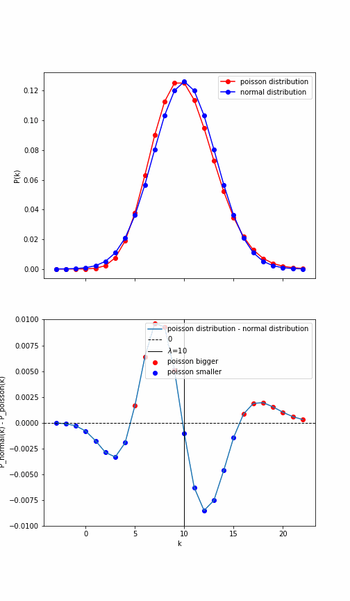
このように、証明は私にはよく分からないが、ポアソン分布と正規分布の差は$\lambda$に反比例しているのである。
一方、正規分布の最大値は、

{\displaystyle f(\mu)={\frac {1}{\sqrt {2\pi \sigma ^{2}}}}}

となり、$\sigma$に反比例していることが分かる。$\sigma =\sqrt{\lambda}$より、2つの分布の差は$\lambda$に反比例、2つの分布の見た目は$\sqrt{\lambda}$に反比例するので、ただ差が小さくなるだけでなく見た目の差も小さくなると考えられる。上のGIF動画を見ても$\lambda$が大きくなると相対的な2つの分布の差(GIF動画の1つ目の図)が小さく見えることがわかる。
実際に$y_1=1/x \cdot \sqrt{x}$と$y_2=1/\sqrt{x} \cdot \sqrt{x}$をグラフにプロットするとよく理解できる。最後の$\sqrt{x}$を掛ける気持ちは、$\sqrt{x}$倍して上のGIF動画の1つ目の図の見た目と同じ処理をしている。

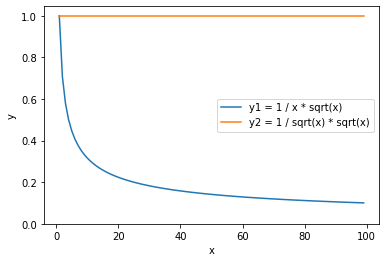
ところで、橙色は2つの分布そのものであるから、$\lambda$によらず見た目は変わらないのは当たり前である。一方、水色は2つの分布の差であるため、このように$1/x$で小さくなる。つまり、$\lambda$が大きくなるに連れて2つの分布の見た目の差は、$1/\lambda$で小さくなることがわかる。

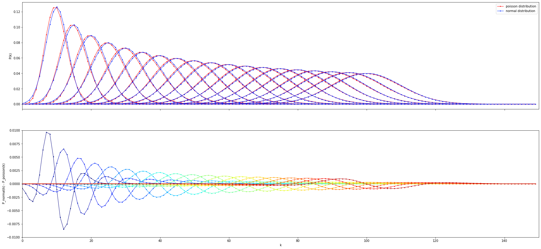
おまけ

$\lambda$を10-100まで5刻みに変えたときの、ポアソン分布と正規分布の差を重ねてプロットしたものである。色は青から赤にかけて$\lambda$の増加を表す。

lambda_s = np.arange(10, 101, 5)
ks = np.arange(0, 150, 1)

fig, (ax1, ax2) = plt.subplots(figsize=(30, 14), nrows=2, sharex=True)
for i, lambda_ in enumerate(lambda_s):
    # ポアソン分布、正規分布、ポアソン分布 - 正規分布の計算
    sigma = np.sqrt(lambda_)
    poisson_distribution = poisson.pmf(ks, lambda_)
    normal_distribution = norm.pdf(ks, loc=lambda_, scale=sigma)
    diffs = poisson_distribution - normal_distribution

    # ポアソン分布, 正規分布、ポアソン分布 - 正規分布をプロット
    poisson_plot, = ax1.plot(ks, poisson_distribution, 'o-', c='red', lw=1, markersize=2)
    normal_plot, = ax1.plot(ks, normal_distribution, 'o-', c='blue', lw=1, markersize=2)
    ax2.plot(ks, diffs, 'o-', c=cm.jet(i / lambda_s.shape[0]), lw=1, markersize=2)

ax1.set_ylabel('P(k)')
ax1.legend([poisson_plot, normal_plot], ['poisson distribution', 'normal distribution'], loc='upper right')

ax2.set_xlim(0, 150)
ax2.set_ylim(-0.01, 0.01)
ax2.set_xlabel('k')
ax2.set_ylabel(' P_normal(k) - P_poisson(k)')

plt.show()

まとめ

ポアソン分布と正規分布は近似できると良く言われているが、ただ近似できると言われても納得できない方やどのように近似されるのかグラフを通して理解したい方向けの記事を書きました。
2つの分布の差が小さくなるだけでなく見た目の差も小さくなるところが面白いですね。
可視化してわかる世界を堪能していただけたら幸いです。

ポアソン分布が正規分布に近づく様子を可視化して理解しよう

概要

実装

各種インポート

ポアソン分布と正規分布の比較

lambda_=10

lambda_=20

lambda_=100

考えられる性質

おまけ

まとめ