【matplotlib】画素数の大きいイメージの表示・保存は、figsizeまたはdpiを大きめに設定しないとまずい

はじめに

まず、下のgifをご覧いただきたい。ランダムな0, 1のみで構成された2次元配列をmatplotlibでカラーを付けて表示したものである。白黒画像になってほしいがピクセルサイズを大きくすると途中から赤くなる。

さらに進めていくと赤い網目が出てくる。このように、画素数が大きすぎて表示できないイメージはmatplotlib流の誤魔化し方で表現しているのである。

概要

matplotlibのimshowで画素数の大きなイメージを作成し、解像度を上げずに表示したときの挙動を確認した。

方法

乱数を使い0と1のみのランダムな値の入った2次元配列を生成する。matplotlibのimshowで生成された2次元配列を読み込み、最小値0、最大値1のカラーバーで表示する。

ランダムな0,1のみの2次元配列を図に表示

import numpy as np
import random
import matplotlib.pyplot as plt
from mpl_toolkits.axes_grid1 import make_axes_locatable


def get_random_image(px_size):
    random.seed(10)  # 再現性のため乱数の種を指定
    image = np.zeros([px_size, px_size])
    for y in range(px_size):
        for x in range(px_size):
            rand = random.randrange(2)  # 0, 1の乱数を生成
            image[y][x] = rand
    return image

px_size = 260  # px_sizeの指定
image = get_random_image(px_size)  # px_size×px_sizeのimageを作成

fig = plt.figure(figsize=(5, 5), dpi=72)
ax = fig.add_subplot(1, 1, 1)
color = ax.imshow(image, vmin=0, vmax=1, cmap='CMRmap')
divider = make_axes_locatable(ax)
cax = divider.append_axes('right', size='5%', pad=0.05)
ax.set_title('px_size={}'.format(px_size))
ax.set_aspect('equal')
ax.axis('off')
plt.colorbar(color, cax=cax)
plt.show()

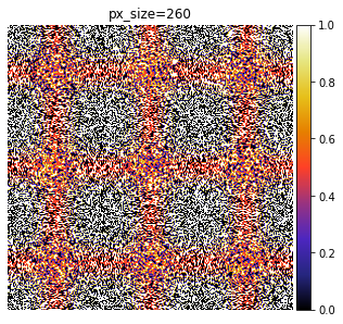
表示される画像。白黒画像が期待されるが、赤い網目が見える。

解決策

解像度を上げることで解決できる。解像度を上げるには、figsizeまたはdpiを大きくする。
figsizeまたはdpiの関係は、matplotlib – 指定した解像度で図を保存する方法についてを参照されたい。
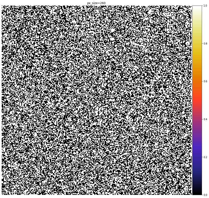
figsizeを大きくした例を示す。

fig = plt.figure(figsize=(5, 5), dpi=72)の画像。

fig = plt.figure(figsize=(14.8, 14.8), dpi=72)の画像。

おまけ

以下の項目を見ていきます。ただし、間違った解釈をする恐れがあるため、matplotlib流の誤魔化し方について考察はせず、得られた結果のみを紹介します。コードはGoogle Colaboratoryこちらにあります。

• px_size1-300までのgif（ファイルサイズが大きくQiitaに投稿できなかったため、Google Colab内で紹介）
• 赤い網目の出現箇所の挙動
• matplotlib流の誤魔化し方を追う
  • 黒のみとそれ以外に分解
  • 白黒以外のピクセルの総数を計算
  • 0, 1（白黒）の配合比を変更したときの挙動

赤い網目の出現箇所の挙動

px_sizeを1から1000まで確認したところ、132と263の2箇所で赤い網目の構造が確認できた。
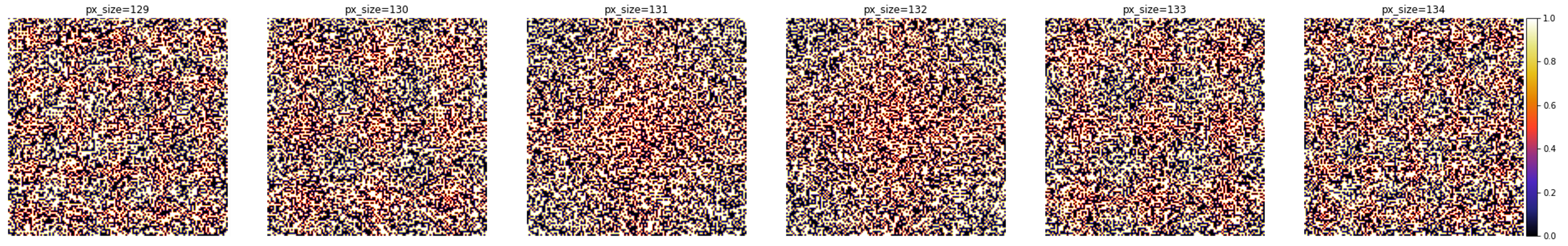
px_sizeが129-134までの図を示す。px_sizeが1変化するごとに網目が2つ増減していることが確認できる。

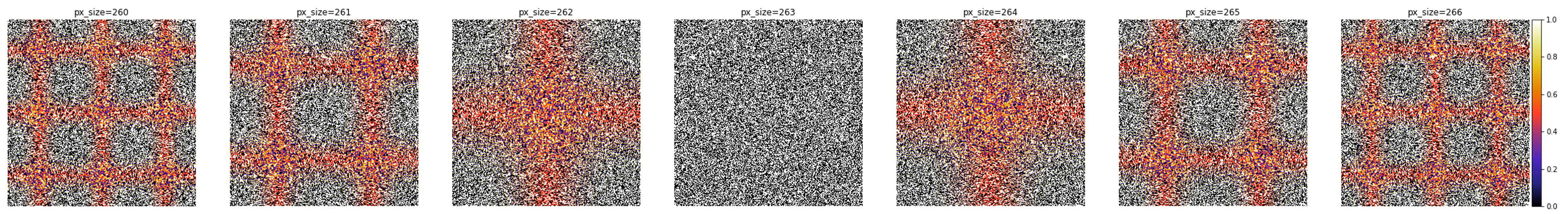
px_sizeが260-266までの図を示す。px_sizeが1変化するごとに網目が1つ増減していることが確認できる。また、px_sizeが263で白黒画像になる。

matplotlib流の誤魔化し方を追う

黒のみとそれ以外に分解

pngで保存（px_size=260の例）

import numpy as np
import random
import matplotlib.pyplot as plt
from mpl_toolkits.axes_grid1 import make_axes_locatable


def get_random_image(px_size):
    random.seed(10)  # 再現性のため乱数の種を指定
    image = np.zeros([px_size, px_size])
    for y in range(px_size):
        for x in range(px_size):
            rand = random.randrange(2)  # 0, 1の乱数を生成
            image[y][x] = rand
    return image

px_size = 260  # px_sizeの指定
image = get_random_image(px_size)  # px_size×px_sizeのimageを作成

fig = plt.figure(figsize=(5, 5), dpi=72)
ax = fig.add_subplot(1, 1, 1)
color = ax.imshow(image, vmin=0, vmax=1, cmap='CMRmap')
divider = make_axes_locatable(ax)
cax = divider.append_axes('right', size='5%', pad=0.05)
ax.set_title('px_size={}'.format(px_size))
ax.set_aspect('equal')
ax.axis('off')
plt.colorbar(color, cax=cax)
plt.savefig('0260.png')  # pngで保存
plt.close()

保存したファイルを読み込み、黒のみとそれ以外に分解する。

黒のみとそれ以外に分解（px_size=260の例）

import numpy as np
import random
from matplotlib.image import imread
import matplotlib.pyplot as plt
from mpl_toolkits.axes_grid1 import make_axes_locatable


image = imread('0260.png')  # px_size=260のpngを読み込む
y_range, x_range, value = image.shape
image_black_only = np.ones([y_range, x_range, value])  #value=[1, 1, 1, 1]で初期化
image_excluding_black = np.ones([y_range, x_range, value])  #value=[1, 1, 1, 1]で初期化
black = np.array([0, 0, 0, 1])  #黒=[R:赤, G:緑, B:青, A:透明度]=[0, 0, 0, 1]
for y in range(y_range,):
    for x in range(x_range):
        if x < 311 and y > 44:  #タイトルとcolorbar以外を読み込む
            image_y_x = image[y][x]
            if (image_y_x == black).all():  #黒のみを抽出
                image_black_only[y][x] = image_y_x
            else:
                image_excluding_black[y][x] = image_y_x

fig = plt.figure(figsize=(18, 42), dpi=72)
title_list = ['image_black_only', 'image_excluding_black', 'image_black_only + image_excluding_black']
image_list = [image_black_only, image_excluding_black, image]
for i, (title, image) in enumerate(zip(title_list, image_list)):
    ax = fig.add_subplot(1, 3, i+1)
    ax.imshow(image)
    ax.set_title(title)
    ax.axes.xaxis.set_visible(False)
    ax.axes.yaxis.set_visible(False)
    plt.gca().spines['right'].set_visible(False)
    plt.gca().spines['top'].set_visible(False)
    plt.gca().spines['left'].set_visible(False)
    plt.gca().spines['bottom'].set_visible(False)
plt.show()

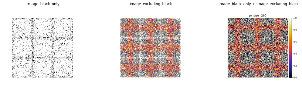
px_size=260で表示される画像。image_black_onlyの図から、黒い網目が見える。

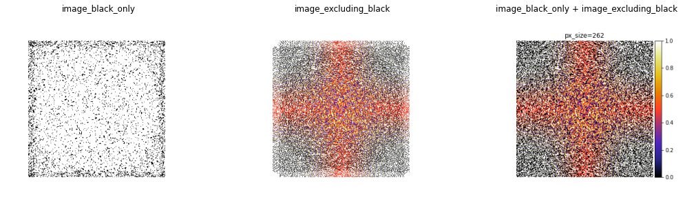
px_size=262で表示される画像。image_black_onlyの図から、プロットエリアの正方形の一辺を直径とする円が見え、円内は黒色の割合が少ないことが分かる。

白黒以外のピクセルの総数を計算

白黒以外のピクセルの総数を計算（px_size=260の例）

import numpy as np
from matplotlib.image import imread


image = imread('0260.png')  # px_size=260のpngを読み込む
y_range, x_range, _ = image.shape
white = np.array([1, 1, 1, 1])  #白=[R:赤, G:緑, B:青, A:透明度]=[1, 1, 1, 1]
black = np.array([0, 0, 0, 1])  #黒=[R:赤, G:緑, B:青, A:透明度]=[0, 0, 0, 1]
count_others = 0
for y in range(y_range):
    for x in range(x_range):
        if x < 311 and y > 44:  #タイトルとcolorbar以外を読み込む
            image_y_x = image[y][x]
            #白黒以外を抽出
            if not ((image_y_x == white).all() or (image_y_x == black).all()):
                count_others += 1

print('白黒以外のピクセルの総数は、{}個'.format(count_others))

出力結果は、白黒以外のピクセルの総数は、54361個となる。
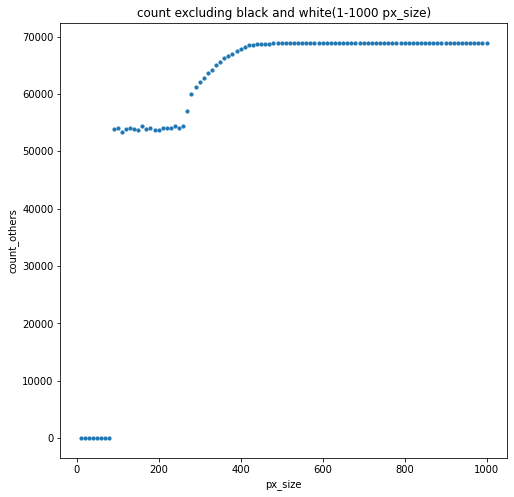
px_sizeを10刻みで横軸をpx_size、縦軸をcount_others（白黒以外のピクセルの総数）でグラフにプロットした。

px_size1-1000まで10刻みで保存

import numpy as np
import random
import matplotlib.pyplot as plt
from mpl_toolkits.axes_grid1 import make_axes_locatable


def get_random_image(px_size):
    random.seed(10)  # 再現性のため乱数の種を指定
    image = np.zeros([px_size, px_size])
    for y in range(px_size):
        for x in range(px_size):
            rand = random.randrange(2)  # 0, 1の乱数を生成
            image[y][x] = rand
    return image


for px_size in range(10, 1001, 10):  # px_sizeの指定
    image = get_random_image(px_size)  # px_size×px_sizeのimageを作成

    fig = plt.figure(figsize=(5, 5), dpi=72)
    ax = fig.add_subplot(1, 1, 1)
    color = ax.imshow(image, vmin=0, vmax=1, cmap='CMRmap')
    divider = make_axes_locatable(ax)
    cax = divider.append_axes('right', size='5%', pad=0.05)
    ax.set_title('px_size={}'.format(px_size))
    ax.set_aspect('equal')
    ax.axis('off')
    plt.colorbar(color, cax=cax)
    plt.savefig('{:0>4}'.format(px_size)) #右寄せ0埋め4桁pngで保存（例：0010, 0260）
    plt.close()

白黒以外のピクセルの総数のグラフ

import numpy as np
from matplotlib.image import imread


px_size_list = list(range(10, 1001, 10))  # 横軸
count_others_list = []  # 縦軸
white = np.array([1, 1, 1, 1])  #白=[R:赤, G:緑, B:青, A:透明度]=[1, 1, 1, 1]
black = np.array([0, 0, 0, 1])  #黒=[R:赤, G:緑, B:青, A:透明度]=[0, 0, 0, 1]
for px_size in px_size_list:
    image = imread('{:0>4}.png'.format(px_size)) #pngを読み込む
    y_range, x_range, _ = image.shape
    count_others = 0  # count計算の初期化
    for y in range(y_range):
        for x in range(x_range):
            if x < 311 and y > 44:  #タイトルとcolorbar以外を読み込む
                image_y_x = image[y][x]
                #白黒以外を抽出
                if not ((image_y_x == white).all() or (image_y_x == black).all()):
                    count_others += 1
    count_others_list.append(count_others)

fig = plt.figure(figsize=(8, 8), dpi=72)
ax = fig.add_subplot(1, 1, 1)
ax.scatter(px_size_list, count_others_list, s=10, marker='o')
ax.set_title('count excluding black and white(1-1000 px_size)')
ax.set_xlabel('px_size')
ax.set_ylabel('count_others') 
plt.show()

表示される画像。

• px_size10-80では、count_othersは0となる。
• px_size80-90では、count_othersは54000程度増加する。
• px_size90-300付近では、count_othersは1000程度のばらつきを持ち一定となる。
• px_size300-500付近にかけて、count_othersは14000程度増加する。
• px_size500-1000付近では、count_othersはほぼ一定の値を取る。（白黒が完全になくなっていく。）

0, 1（白黒）の配合比を変更したときの挙動

0,1の配合比の変更（px_size=260,black_ratio=2の例）

import numpy as np
import random
import matplotlib.pyplot as plt
from mpl_toolkits.axes_grid1 import make_axes_locatable


def get_unbalance_random_image(px_size, black_ratio):
    random.seed(10)  # 再現性のため乱数の種を指定
    image = np.zeros([px_size, px_size])
    for y in range(px_size):
        for x in range(px_size):
            rand = random.randrange(10)  # 0-10の乱数を生成
            if rand < black_ratio:  #black_rationに従い0, 1に分ける
                image[y][x] = 0
            else:
                image[y][x] = 1
    return image


px_size = 260  # px_sizeの指定
black_ratio = 2  # black_ratioは、全体を10としたときの割合
image = get_unbalance_random_image(px_size, black_ratio)

fig = plt.figure(figsize=(5, 5), dpi=72)
ax = fig.add_subplot(1, 1, 1)
color = ax.imshow(image, vmin=0, vmax=1, cmap='CMRmap')
divider = make_axes_locatable(ax)
cax = divider.append_axes('right', size='5%', pad=0.05)
ax.set_title('px_size={}, black:white={}:{}'.format(px_size, black_ratio, 10 - black_ratio))
ax.set_aspect('equal')
ax.axis('off')
plt.colorbar(color, cax=cax)
plt.show()

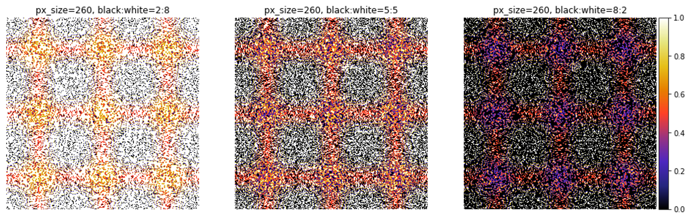
px_size=260で表示される画像。

• 網目の色
  • 黒:白=2:8, 5:5, 8.2では全て赤色(0.5程度)、白色(1.0程度)、黒色(0.0程度)
• 網目の交点付近の色
  • 黒:白=2:8では黄色(0.8程度)
  • 黒:白=5:5では赤色(0.5程度)
  • 黒:白=8:2では青色(0.2程度)

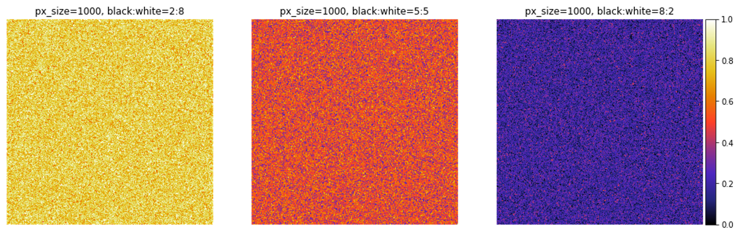
px_size=1000で表示される画像。

• 全体の色
  • 黒:白=2:8では黄色(0.8程度)
  • 黒:白=5:5では赤色(0.5程度)
  • 黒:白=8:2では青色(0.2程度)
• 他に見える色
  • 黒:白=2:8では白色(1.0程度)、赤色(0.5程度)
  • 黒:白=5:5では青色(0.5程度)、黄色(0.8程度)
  • 黒:白=8:2では黒色(0.0程度)、赤色(0.5程度)

まとめ

matplotlibで画素数の大きいイメージを表示・保存するときは、解像度に注意しましょう。