天体画像解析における方位角依存Radial Profileの実装

はじめに

天体画像の解析において、中心からの強度分布を調べるRadial Profile（放射状プロファイル）は、天体の空間構造を理解するうえで基本的かつ有効な手法の一つです。通常のRadial Profileでは、全方位にわたる円環の平均を取得しますが、対象が非対称な場合や、特定の方向に構造がある場合（例：ジェット、衝撃波、非等方性など）には、それでは重要な特徴が埋もれてしまうことがあります。

そこで本記事では、任意の方位角範囲を指定してRadial Profileを取得するPython関数を実装し、擬似画像や実際の観測データを用いた解析例を通して、その使い方を紹介します。

なお、本記事ではカウント画像（光子統計）を前提としており、Radial Profileにおける誤差は統計誤差（ポアソン誤差）を想定しています。

本記事のコードはGoogle Colabこちらからもご覧いただけます。

---

また、天体画像に特化したRadial Profileの解説については、以下の記事でも詳しく取り上げています。よろしければあわせてご覧ください。

Radial Profile関数の実装

import numpy as np
import matplotlib.pyplot as plt
import matplotlib as mpl
from matplotlib.colors import LogNorm
from matplotlib import colormaps
from matplotlib.colors import LinearSegmentedColormap, ListedColormap
from astropy.io import fits
from astropy.wcs import WCS
from astropy.coordinates import SkyCoord

np.random.seed(2025)
plt.rcParams['font.size'] = 12

def calculate_radial_profile(image, center, radius, angle_ranges, binsize=1):
    if binsize < 1:
        raise ValueError(f"binsize must be >= 1, but got {binsize}")
    y, x = np.indices(image.shape)
    cx, cy = center

    # 中心からの距離と角度を計算
    r = np.sqrt((x - cx)**2 + (y - cy)**2)
    theta = np.rad2deg(np.arctan2(y - cy, x - cx)) % 360

   # 全角度範囲をカバーするかチェック
    covers_full_circle = any(
        abs(angle_range[1] - angle_range[0]) >= 360
        for angle_range in angle_ranges
    )

    # 360度以上の場合は全体マスクを適用
    if covers_full_circle or len(angle_ranges) == 0:
        angle_mask = np.ones_like(theta, dtype=bool)
    else:
        angle_mask = np.zeros_like(theta, dtype=bool)
        for angle_range in angle_ranges:
            angle_start = angle_range[0] % 360
            angle_end = angle_range[1] % 360

            if angle_start <= angle_end:
                angle_mask |= (theta >= angle_start) & (theta <= angle_end)
            else:
                angle_mask |= (theta >= angle_start) | (theta <= angle_end)

    # 半径と方位角でマスクを作成
    mask = ((r <= radius) & angle_mask) | (r == 0)

    # マスクを適用した一次元配列
    masked_image = image[mask]

    # 距離をビン分け
    bins = int(radius / binsize)
    radial_bins = np.linspace(0, radius, bins+1)
    bin_indices = np.digitize(r[mask], radial_bins) - 1

    # 各ビンにおける平均値と誤差を計算
    radial_profile = np.zeros(bins)
    poisson_error = np.zeros(bins)

    for i in range(bins):
        values_in_bin = masked_image[bin_indices == i]
        if len(values_in_bin) > 0:
            # 平均値
            radial_profile[i] = values_in_bin.mean()
            # ポアソン誤差
            sum_in_bin = values_in_bin.sum()
            poisson_error[i] = np.sqrt(sum_in_bin) / len(values_in_bin)
        else:
            radial_profile[i] = np.nan
            poisson_error[i] = np.nan

    # デバッグ用のmask領域
    mask_region = np.full_like(image, np.nan, dtype=float)
    mask_region[mask] = 1

    # 各ビンの中央の値を取得
    bin_centers = (radial_bins[:-1] + radial_bins[1:]) / 2

    return bin_centers, radial_profile, poisson_error, mask_region

引数一覧

引数	型	説明
image	2D ndarray	2次元の画像データ。image[y, x] の形式で、横軸がx（列方向）、縦軸がy（行方向）に対応
center	tuple of float	中心座標。形式は (x, y)。ただしNumPy配列では image[y, x] の順番なので注意
radius	float	解析する最大の半径（ピクセル単位）
angle_ranges	list of tuple	方位角の範囲をリストで指定。例：[(30, 60)] や [(0, 45), (315, 360)] など。複数範囲を指定すると、それらを統合して1つの領域として扱われる
binsize	float	半径方向のビンサイズ（省略時は1ピクセル単位）。1未満の値は、ピクセルが含まれないビンが生じうるため、この関数では使用不可（エラーになります）

戻り値一覧

戻り値	型	説明
bin_centers	1D ndarray	各ビンの中心に対応する半径（ピクセル単位）
radial_profile	1D ndarray	各ビンにおける平均強度（指定された方位角範囲内で平均化）
poisson_error	1D ndarray	各ビンのポアソン誤差（$\sqrt{N}/N$）
mask_region	2D ndarray	デバック用の解析に使われた領域を示すマスク画像（使われた画素は1、それ以外はNaN）

使い方

ここでは、先ほど実装した calculate_radial_profile() 関数の基本的な使い方と応用例を、擬似データを用いたプロット付きで丁寧に解説していきます。

擬似観測画像の用意

デモンストレーション用に適当なガウシアン分布を用意します。

模擬的な観測画像を生成

image_size = 201
sigma = 20

image = np.zeros((image_size, image_size))
cx, cy = image.shape[1] // 2, image.shape[1] // 2  # 点源の位置
x, y = np.meshgrid(np.arange(image_size), np.arange(image_size))
image = 50 * np.exp(-((x - cx)**2 + (y - cy)**2) / (2 * sigma**2))
image = np.random.poisson(image)

基本の使い方（全方位平均）

まずは、シンプルなケースとして、たとえば、0°から360°の通常のRadial Profileを取得する場合、以下のように関数を利用できます。

# Radial Profileのパラメータ
center = (100, 100)
radius = 80
binsize = 1
angle_range = (0, 360)
angle_ranges = [angle_range]
radial_bins, radial_profile, poisson_error, mask_region = calculate_radial_profile(image, center, radius, angle_ranges, binsize)

# プロットのセットアップ
fig, axes = plt.subplots(1, 3, figsize=(18, 6))

# 左: 元画像
axes[0].imshow(image, origin='lower', cmap='gray')
axes[0].set_title("Original Image")
axes[0].set_xlabel("x (px)")
axes[0].set_ylabel("y (px)")

# 中央: Radial Mask Image
axes[1].imshow(image*mask_region, origin='lower', cmap='gray')
axes[1].set_title("Masked Radial Image")
axes[1].plot(center[0], center[1], 'x', color='lime', label='Center')
axes[1].set_xlabel("x (px)")
axes[1].set_ylabel("y (px)")
axes[1].legend()

# 右: Radial Profile
axes[2].errorbar(radial_bins, radial_profile, yerr=poisson_error, fmt='.')
axes[2].set_title("Radial Profile")
axes[2].set_xlabel("Radius (px)")
axes[2].set_ylabel("Average Intensity")
axes[2].grid()

plt.show()

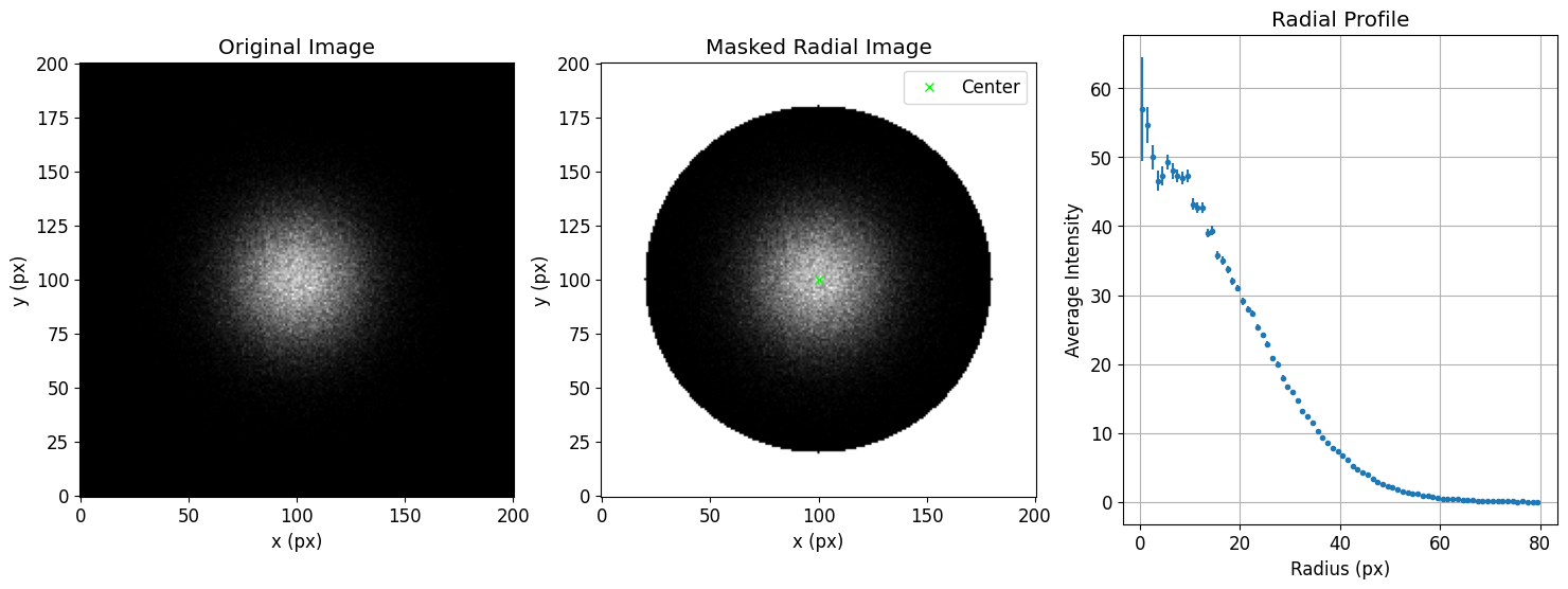
左から、観測画像、観測画像にプロファイルのマスクを適用した画像、Radial Profileになります。中央の画像のクロスはプロファイルを計算する際に使用した中心位置を示しています。

方位角を指定した使い方

1. 0°～30°

0°~30°

center = (100, 100)
radius = 80
binsize = 1
angle_range = (0, 30)
angle_ranges = [angle_range]
radial_bins, radial_profile, poisson_error, mask_region = calculate_radial_profile(image, center, radius, angle_ranges, binsize)

2. -30°～60°

本関数は負の角度や360°を超える角度指定にも対応しています。

-30°～60°

center = (100, 100)
radius = 80
binsize = 1
angle_range = (-30, 60)  # (330, 420)などの角度表記でも指定可能
angle_ranges = [angle_range]
radial_bins, radial_profile, poisson_error, mask_region = calculate_radial_profile(image, center, radius, angle_ranges, binsize)

3. 複数範囲の指定

複数の異なる角をまとめてリストにすると、それらを統合したプロファイルが得られます。

center = (100, 100)
radius = 80
binsize = 1
angle_range_1 = (-10, 30)
angle_range_2 = (170, 210)
angle_ranges = [angle_range_1, angle_range_2]  # 複数をリストで指定
radial_bins, radial_profile, poisson_error, mask_region = calculate_radial_profile(image, center, radius, angle_ranges, binsize)

ビンサイズの変更

Radial Profileでは、ビンサイズの設定が結果に大きく影響します。

小さいビンサイズは構造を細かく捉えられますが、統計誤差が大きくなります。一方、大きいビンは誤差を抑えられるものの、細かな構造が平均化されて見えにくくなることがあります。

解析対象や目的に応じて、適切なビンサイズを選ぶことが大切です。

binsizeが1未満の場合
本関数では、binsizeが1未満の値を使用できないようにしています。通常の画像では、ビン内にデータが全く存在しない領域が発生する可能性があるためです。これを回避するには、ピクセル以下のスケールを補間やスムージングなどで補正する必要がありますが、それは本記事のスコープを超えるため、ここでは扱いません。

binsize=1, 4, 16の例

# Radial Profileのパラメータ
center = (100, 100)
radius = 80
angle_range = (0, 10)
angle_ranges = [angle_range]
binsizes = [1, 4, 16]

# プロットセットアップ（
fig, axes = plt.subplots(1, 3, figsize=(18, 6))

for i, binsize in enumerate(binsizes):
    radial_bins, radial_profile, poisson_error, mask_region = calculate_radial_profile(
        image, center, radius, angle_ranges, binsize
    )

    axes[0].imshow(image, origin='lower', cmap='gray')
    axes[1].imshow(image * mask_region, origin='lower', cmap='gray')
    axes[2].errorbar(radial_bins, radial_profile, xerr=binsize / 2, yerr=poisson_error, fmt='.', label=f'(binsize={binsize})', alpha=0.7)

axes[0].set_title(f"Original Image")
axes[0].set_xlabel("x (px)")
axes[0].set_ylabel("y (px)")

axes[1].plot(center[0], center[1], 'x', color='lime', label='Center')
axes[1].set_title(f"Masked Radial Image")
axes[1].set_xlabel("x (px)")
axes[1].set_ylabel("y (px)")
axes[1].legend()

axes[2].set_title(f"Radial Profile")
axes[2].set_xlabel("Radius (px)")
axes[2].set_ylabel("Average Intensity")
axes[2].grid()
axes[2].legend()

plt.show()

右側の画像のbinsize=1, 4, 16ピクセルの結果ですが、ビンサイズが大きいほど統計誤差の影響が小さくなる反面、動径方向の誤差は大きくなっていることがわかります。

おまけ

方位角毎の描画

ここでは、方位角を一定のステップで分割し、それぞれの範囲に対するRadial Profileを一括で描画する実装例を紹介します。

# Radial Profileのパラメータ
center = (100, 100)
radius = 80
binsize = 1
angle_step = 45  # 各Radial Profileの角度
num_profile = int(360/angle_step)
colors = plt.cm.hsv(np.linspace(0, 1, num_profile, endpoint=False))  # 色を生成（HSVカラーマップ）

# プロットのセットアップ
fig, axes = plt.subplots(1, 3, figsize=(18, 6))

# 各angle_rangeに対して計算しプロット
for i in range(num_profile):
    # 現在のangle_rangeを設定
    angle_range = (angle_step*i, angle_step*(i+1))
    angle_ranges = [angle_range]

    # Radial Profileを計算
    radial_bins, radial_profile, poisson_error, mask_region = calculate_radial_profile(image, center, radius, angle_ranges, binsize)

    # 方位角範囲を色分けして円弧を描画
    angles = np.linspace(angle_range[0], angle_range[1], 100)
    x_arc = center[0] + radius * np.cos(np.deg2rad(angles))
    y_arc = center[1] + radius * np.sin(np.deg2rad(angles))
    axes[1].plot(x_arc, y_arc, color=colors[i], linestyle='-')

    # 方位角範囲を視覚化するための線を描画
    for angle in angle_range:
        x_end = center[0] + radius * np.cos(np.deg2rad(angle))
        y_end = center[1] + radius * np.sin(np.deg2rad(angle))
        axes[1].plot([center[0], x_end], [center[1], y_end], color=colors[i], linestyle='--', alpha=0.7)

    # Radial Profileを右のプロットに追加
    axes[2].errorbar(radial_bins, radial_profile, xerr=binsize/2, yerr=poisson_error, label=f"{angle_range[0]}°-{angle_range[1]}°", color=colors[i], fmt='.')


# 左: 元画像
axes[0].imshow(image, origin='lower', cmap='gray')
axes[0].set_title("Original Image")
axes[0].set_xlabel("x (px)")
axes[0].set_ylabel("y (px)")

# 中央: Radial Mask Image
axes[1].imshow(image, origin='lower', cmap='gray')
axes[1].set_title("Masked Radial Image")
axes[1].plot(center[0], center[1], 'x', color='lime', label='Center')
axes[1].set_xlabel("x (px)")
axes[1].set_ylabel("y (px)")
axes[1].legend()

# 右: Radial Profile
axes[2].set_title("Radial Profile")
axes[2].set_xlabel("Radius (px)")
axes[2].set_ylabel("Average Intensity")
axes[2].grid()
axes[2].legend(title='Angle (degrees)', loc='upper right')

# カラーマップと正規化
cmap = plt.cm.hsv
norm = mpl.colors.Normalize(vmin=0, vmax=360)
sm = mpl.cm.ScalarMappable(cmap=cmap, norm=norm)
sm.set_array([]) 
cbar = fig.colorbar(sm, ax=axes[2], aspect=50)
cbar.set_label("Angle (degrees)")

plt.show()

上の例では、30°ずつのRadial Profileを色分けして表示しています。カラーマップにはHSVを使用しており、各方位角範囲を視覚的に区別しやすくしています。
凡例が多くなる場合は、カラーバーで表示するなど使い分けて活用ください。

超新星残骸カシオペア座Aへの適用例

最後に、Chandra X線衛星が2004年に観測した超新星残骸カシオペア座A（Cassiopeia A）の実データを用いて、Radial Profileの解析を行ってみます。

以下のリンクから、事前にObservation ID 4636, 4637, 4639, 5319のデータをCIAOツールで校正・統合した2–7 keV帯のFITS画像をダウンロードできます。

• 2004_hard_thresh.expmap: エクスポージャーマップ（単位: cm² s count / photon）
• 2004_hard_thresh.img: 光子数マップ（単位: count）

この解析では、本記事で紹介した関数をベースにしつつ、露光補正（exposure correction）を導入したバージョンを使用しています。

カシオペア座Aへの適用

# DS9 bカラーマップの登録
# DS9カラーマップの記事：https://qiita.com/yusuke_s_yusuke/items/b30ca36be1c43beecde5
cmap_name = 'ds9_b'
cmap_r_name = f'{cmap_name}_r'

# まだ登録されていなければ登録
if cmap_name not in colormaps:
    ds9_b_cdict = {
        'red':   [(0.0, 0.0, 0.0), (.25, 0.0, 0.0), (.5, 1.0, 1.0), (1.0, 1.0, 1.0)],
        'green': [(0.0, 0.0, 0.0), (.5, 0.0, 0.0), (.75, 1.0, 1.0), (1.0, 1.0, 1.0)],
        'blue':  [(0.0, 0.0, 0.0), (.25, 1.0, 1.0), (.5, 0.0, 0.0), (.75, 0.0, 0.0), (1.0, 1.0, 1.0)]
    }

    ds9_b_cmap = LinearSegmentedColormap(cmap_name, ds9_b_cdict)
    colormaps.register(name=cmap_name, cmap=ds9_b_cmap)

    ds9_b_r_cmap = ds9_b_cmap.reversed()
    colormaps.register(name=cmap_r_name, cmap=ds9_b_r_cmap)

def calculate_radial_profile_for_chandra(thresh_image, expmap, center, radius, angle_ranges, binsize=1):
    if binsize < 1:
        raise ValueError(f"binsize must be >= 1, but got {binsize}")
    y, x = np.indices(thresh_image.shape)
    cx, cy = center

    # 中心からの距離と角度を計算
    r = np.sqrt((x - cx)**2 + (y - cy)**2)
    theta = np.rad2deg(np.arctan2(y - cy, x - cx)) % 360

   # 全角度範囲をカバーするかチェック
    covers_full_circle = any(
        abs(angle_range[1] - angle_range[0]) >= 360
        for angle_range in angle_ranges
    )

    # 360度以上の場合は全体マスクを適用
    if covers_full_circle or len(angle_ranges) == 0:
        angle_mask = np.ones_like(theta, dtype=bool)
    else:
        angle_mask = np.zeros_like(theta, dtype=bool)
        for angle_range in angle_ranges:
            angle_start = angle_range[0] % 360
            angle_end = angle_range[1] % 360

            if angle_start <= angle_end:
                angle_mask |= (theta >= angle_start) & (theta <= angle_end)
            else:
                angle_mask |= (theta >= angle_start) | (theta <= angle_end)

    # 半径と方位角でマスクを作成
    mask = ((r <= radius) & angle_mask) | (r == 0)

    # マスクを適用した一次元配列
    masked_image = thresh_image[mask]
    masked_expmap = expmap[mask]

    # 距離をビン分け
    bins = int(radius / binsize)
    radial_bins = np.linspace(0, radius, bins+1)
    bin_indices = np.digitize(r[mask], radial_bins) - 1

    # 各ビンにおける平均値と誤差を計算
    radial_profile = np.zeros(bins)
    poisson_error = np.zeros(bins)

    for i in range(bins):
        values_in_bin = masked_image[bin_indices == i]
        expmap_in_bin = masked_expmap[bin_indices == i]
        if len(values_in_bin) > 0:
            sum_values_in_bin = values_in_bin.sum()
            sum_expmap_in_bin = expmap_in_bin.sum()
            radial_profile[i] = sum_values_in_bin / sum_expmap_in_bin
            poisson_error[i] = np.sqrt(sum_values_in_bin) / sum_expmap_in_bin
        else:
            radial_profile[i] = np.nan
            poisson_error[i] = np.nan

    # デバッグ用のmask領域
    mask_region = np.full_like(thresh_image, np.nan, dtype=float)
    mask_region[mask] = 1

    # 各ビンの中央の値を取得
    bin_centers = (radial_bins[:-1] + radial_bins[1:]) / 2

    return bin_centers, radial_profile, poisson_error, mask_region

# FITSファイルの読み込みとWCSの取得
with fits.open("2004_hard_thresh.img") as hdul:
    casa_image = hdul[0].data
    wcs = WCS(hdul[0].header)

with fits.open("2004_hard_thresh.expmap") as hdul:
    casa_expmap = hdul[0].data

# RA/Dec を文字列で渡して SkyCoord に変換
# Cas A の中心座標 Thorstensen et al. 2001
coord = SkyCoord("23h23m27.77s", "+58d48m49.4s", frame="icrs")

# degree に変換
ra_center = coord.ra.deg
dec_center = coord.dec.deg

# RA/Decからピクセル座標に変換
center_pix = wcs.wcs_world2pix([[ra_center, dec_center]], 0)[0]
center = (center_pix[0], center_pix[1])  # (x, y)

# Radial Profileのパラメータ
radius = 480
binsize = 1
angle_step = 60
num_profile = int(360/angle_step)
colors = plt.cm.hsv(np.linspace(0, 1, num_profile, endpoint=False))

# プロットのセットアップ（wcsを使ってRA/Dec表示）
fig = plt.figure(figsize=(18, 6))
axes = [
    fig.add_subplot(1, 3, 1, projection=wcs),
    fig.add_subplot(1, 3, 2, projection=wcs),
    fig.add_subplot(1, 3, 3)
]

# 各angle_rangeに対して計算しプロット
for i in range(num_profile):
    angle_range = (angle_step * i, angle_step * (i + 1))
    angle_ranges = [angle_range]

    radial_bins, radial_profile, poisson_error, mask_region = calculate_radial_profile_for_chandra(
        casa_image, casa_expmap, center, radius, angle_ranges, binsize
    )

    # 円弧の描画
    angles = np.linspace(angle_range[0], angle_range[1], 100)
    x_arc = center[0] + radius * np.cos(np.deg2rad(angles))
    y_arc = center[1] + radius * np.sin(np.deg2rad(angles))
    axes[1].plot(x_arc, y_arc, color=colors[i], linestyle='-')

    for angle in angle_range:
        x_end = center[0] + radius * np.cos(np.deg2rad(angle))
        y_end = center[1] + radius * np.sin(np.deg2rad(angle))
        axes[1].plot([center[0], x_end], [center[1], y_end], color=colors[i], linestyle='--', alpha=0.7)

    # Radial Profile
    axes[2].errorbar(radial_bins, radial_profile, xerr=binsize/2, yerr=poisson_error,
                     label=f"{angle_range[0]}°-{angle_range[1]}°", color=colors[i], fmt='.')

# 左: 元画像（RA/Dec表示）
axes[0].imshow(casa_image, origin='lower', cmap='ds9_b', norm=LogNorm())
axes[0].set_title("Original Image (log)")
axes[0].set_xlabel("RA")
axes[0].set_ylabel("Dec")

# 中央: マスク可視化（RA/Dec表示）
axes[1].imshow(casa_image, origin='lower', cmap='ds9_b', norm=LogNorm())
axes[1].plot(center[0], center[1], 'x', color='lime', label='Center')
axes[1].set_title("Masked Radial Image (log)")
axes[1].legend()
axes[1].set_xlabel("RA")
axes[1].set_ylabel("Dec")

# 右: Radial Profile（ピクセル距離 vs 強度）
axes[2].set_title("Radial Profile")
axes[2].set_xlabel("Radius (px)")
axes[2].set_ylabel("Flux (photon / cm$^2$ / s / pixel)")
axes[2].grid()
axes[2].legend(title="Angle (deg)", loc='upper right')

# カラーバー（角度）
cmap = plt.cm.hsv
norm = mpl.colors.Normalize(vmin=0, vmax=360)
sm = mpl.cm.ScalarMappable(cmap=cmap, norm=norm)
sm.set_array([])
cbar = fig.colorbar(sm, ax=axes[2], aspect=50)
cbar.set_label("Angle (degrees)")

fig.tight_layout()
plt.show()

expmapの役割
X線観測では、CCDチップの位置によって有効面積や露光時間がわずかに異なるため、ピクセルごとの補正が重要です。そのため、calculate_radial_profile_for_chandra()関数では、expmapを使って光子数を正規化し、物理量（flux: photon/cm²/s/pixel）としてのRadial Profileを算出しています。

このように、Radial Profileを方位角ごとに表示することで、超新星残骸のような天体における非対称な構造を可視化・解析することが可能になります。

さらに、複数の観測年のデータを使い、相関を調べることで、膨張速度を調べることもできます（例：Vink et al. 2022)。
こちらで紹介していますので、よろしければご覧ください。

ちなみに天文学でお馴染みのDS9のカラーマップをmatplotlibで再現する方法はこちらで解説していますので、よろしければご覧ください。

まとめ

本記事では、任意の方位角範囲を指定してラディアルプロファイルを解析するPythonスクリプトを紹介し、擬似データや実際の観測データ（超新星残骸カシオペア座A）を用いて、その活用方法を解説しました。
対象天体の非対称性や方向依存性のある構造を、より詳細に解析するための一助となれば幸いです。

関連記事