みなさんこんにちは。
現在、Pythonを勉強している社会人3年目の転職希望者です。
プログラミングスクールに通い、様々な分析手法を学びました。これからは、更に実践で活躍できるようになる為、自らデータを探し、データの分析のみならず基礎から学んでいこうと考えています。
このブログが様々な人の役に立てれば光栄に思います。
さて、本題ですが今回使用するデータセットは下記のとおりです
https://www.kaggle.com/competitions/jpx-tokyo-stock-exchange-prediction
JPXが主催のコンペディションになっています。
ここで、JPXとは何か簡単に説明していきます。
日本取引所グループ(JPX)は、世界最大級の証券取引所である東京証券取引所(TSE)と、デリバティブ取引所である大阪取引所(OSE)および東京商品取引所(TOCOM)を運営する持株会社です。
今回はこのコンペディションのデータを用いて、データの読み込みからデータ手法まで幅広く学んでいきたいと思います。
1.データの読み込み
与えられたデータがかなり多いですが、まずは一番大切だと思うデータから読み込んでいきましょう。
stock_price_data = pd.read_csv("../input/jpx-tokyo-stock-exchange-prediction/supplemental_files/stock_prices.csv")

stock_price_data
"""
  RowId	   Date   SecuritiesCodeOpen High	Low	   Close	Volume	AdjustmentFactor	ExpectedDividend	SupervisionFlag	Target
0	20211206_1301	2021-12-06	1301	2982.0	2982.0	2965.0	2971.0	8900	1.0	NaN	False	-0.003263
1	20211206_1332	2021-12-06	1332	592.0	599.0	588.0	589.0	1360800	1.0	NaN	False	-0.008993
2	20211206_1333	2021-12-06	1333	2368.0	2388.0	2360.0	2377.0	125900	1.0	NaN	False	-0.009963
3	20211206_1375	2021-12-06	1375	1230.0	1239.0	1224.0	1224.0	81100	1.0	NaN	False	-0.015032
4	20211206_1376	2021-12-06	1376	1339.0	1372.0	1339.0	1351.0	6200	1.0	NaN	False	0.002867
...	...	...	...	...	...	...	...	...	...	...	...	...
111995	20220228_9990	2022-02-28	9990	511.0	518.0	509.0	516.0	120600	1.0	NaN	False	-0.013592
111996	20220228_9991	2022-02-28	9991	823.0	825.0	814.0	822.0	16200	1.0	NaN	False	-0.020581
111997	20220228_9993	2022-02-28	9993	1600.0	1622.0	1600.0	1600.0	4000	1.0	NaN	False	0.005762
111998	20220228_9994	2022-02-28	9994	2568.0	2568.0	2540.0	2565.0	9000	1.0	NaN	False	-0.002341
111999	20220228_9997	2022-02-28	9997	731.0	737.0	726.0	734.0	288100	1.0	NaN	False	-0.030014
112000 rows × 12 columns
"""
ここで、それぞれのカラムについての説明を記述していきます
# RowId: Unique ID of price records, the combination of Date and SecuritiesCode.
# ・・・ ある会社の取引の日付と証券コード(SecuritiesCode)を合わせたもの
# Date: Trade date.
# SecuritiesCode: Local securities code.
# Open: First traded price on a day.
# High: Highest traded price on a day.
# Low: Lowest traded price on a day.
# Close: Last traded price on a day.
# Volume: Number of traded stocks on a day.
# ・・・一日の取引銘柄数。
# AdjustmentFactor: Used to calculate theoretical price/volume when split/reverse-split happens (NOT including dividend/allotment of shares).
# ・・・分割・併合時の理論株価・出来高の算出に使用します(配当・増資は含まれません)。
# ExpectedDividend: Expected dividend value for ex-right date. This value is recorded 2 business days before ex-dividend date.
# ・・・権利落ち日の配当予想値。この値は、配当落ち日の2営業日前に記録されます。

# SupervisionFlag: Flag of securities under supervision and securities to be delisted, for more information, please see here.
# Target: Change ratio of adjusted closing price between t+2 and t+1 where t+0 is trade date.
# ・・・t+2 と t+1 の修正終値の変化率(t+0 は取引日)。
ここで、どれくらいの日付のデータがあるか確認していきましょう。
stock_price_data["Date"].unique()

array(['2021-12-06', '2021-12-07', '2021-12-08', '2021-12-09',
       '2021-12-10', '2021-12-13', '2021-12-14', '2021-12-15',
       '2021-12-16', '2021-12-17', '2021-12-20', '2021-12-21',
       '2021-12-22', '2021-12-23', '2021-12-24', '2021-12-27',
       '2021-12-28', '2021-12-29', '2021-12-30', '2022-01-04',
       '2022-01-05', '2022-01-06', '2022-01-07', '2022-01-11',
       '2022-01-12', '2022-01-13', '2022-01-14', '2022-01-17',
       '2022-01-18', '2022-01-19', '2022-01-20', '2022-01-21',
       '2022-01-24', '2022-01-25', '2022-01-26', '2022-01-27',
       '2022-01-28', '2022-01-31', '2022-02-01', '2022-02-02',
       '2022-02-03', '2022-02-04', '2022-02-07', '2022-02-08',
       '2022-02-09', '2022-02-10', '2022-02-14', '2022-02-15',
       '2022-02-16', '2022-02-17', '2022-02-18', '2022-02-21',
       '2022-02-22', '2022-02-24', '2022-02-25', '2022-02-28'],
      dtype=object)
データを見てみると2021年12月6日から2022年2月28日のデータであるとわかります。
ここで注意していきたいのが、dtypeです。文字列型になっていますね。
時系列分析などを行う際、これは必ずといってもいいほど変えなくてはいけないものになります。
文字列からdatetime形にしたい場合はPandasのto_datetime関数を用いるとよいです
実際にコードを書いていきます。
stock_price_data['Date'] = pd.to_datetime(stock_price_data['Date'])
では実際にデータ型をみていきましょう。上手くdatetime形式にすることが出来ました。
stock_price_data["Date"].head()
"""
0   2021-12-06
1   2021-12-06
2   2021-12-06
3   2021-12-06
4   2021-12-06
Name: Date, dtype: datetime64[ns]
"""
stock_price_dataは、様々な企業の株価の変動が記載されていることから、どの会社がデータの日付分どのような動きになっているか分かりづらいと思います。
そこで、ある会社のデータのみ見ていきましょう。
私はユニクロが好きなので、なんとなくユニクロの証券コード(9983)を用いてデータを作成していきます。
df = df_train_stock[df_train_stock['SecuritiesCode'] == 9983]
df["Close_shift1"] = df["Close"].shift(-1)
df["Close_shift2"] = df["Close"].shift(-2)

df["rate"] = (df["Close_shift2"] - df["Close_shift1"]) / df["Close_shift1"]
df
一行目は、データフレームにする為に、df_train_stock[]でもう一度囲むことに注意が必要です。
shift(-1)で一個後のデータを抽出することが可能です。
shift(-2)で一個後のデータを抽出することもできます。
それぞれを後と前の差と前のデータから、変化率を抽出しています。
このデータを見てみると、Targetとrateが一致していることが分かります。
このターゲットがとても大切な数値なものであると考察します。
では、このTargetがをヒストグラムで表してみます。
import matplotlib.pyplot as plt
plt.hist(stock_price_data["Target"] ,  bins=1000, range=[-0.2,0.2])
plt.title("Target distribution", weight='bold', fontsize=16)![download.png]
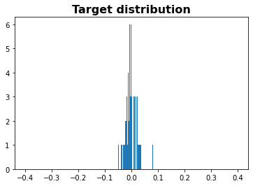
-0.1から+0.1で収束していることが見受けられます。
これから様々な分析をしていきますので、よろしくお願い申し上げます。