0. はじめに
機械学習において、ある分類器を用いて2クラス分類をした際のその分類器の良さを表す指標として、ROC曲線や、そのROC曲線の**AUC(Area Under the Curve:曲線下面積)**が用いられます。
ざっくりと説明すると、
ROC曲線は「その分類器を用いることで、2つの分布をどれだけ切り離すことができたか」を表します。また、AUCという量を用いることで、複数のROC曲線を比較することができます。
学習に用いたモデルによって、ROC曲線を描けるものと描けないものがあります。
model.predict() などを用いたときに出力(返り値)が確率で与えられるようなモデルはROC曲線を描けますが、出力が2値になるようなモデルではROC曲線は描けません。
今回は、scikit-learn を使ってこのROC曲線で遊んでみようと思います。
1. とりあえずデータを用意してみる
冒頭でも述べた通り、出力が確率的なものでしかROC曲線は描けないので、そのような出力を想定します。
すると、以下のような y_true や y_pred が手元にあることになります。
%matplotlib inline
import matplotlib.pyplot as plt
import numpy as np
import pandas as pd
from sklearn import metrics
y_true = [0, 0, 0, 0, 0, 0, 0, 0, 0, 0,
          1, 1, 1, 1, 1, 1, 1, 1, 1, 1]

y_pred = [0.1, 0.15, 0.2, 0.25, 0.3, 0.35, 0.4, 0.5, 0.65, 0.7,
         0.35, 0.45, 0.5, 0.55, 0.6, 0.65, 0.7, 0.75, 0.8, 0.9]

df = pd.DataFrame({'y_true':y_true, 'y_pred':y_pred})
df

データフレームにすると上記のようになります。
これの分布を可視化してみましょう。
x0 = df[df['y_true']==0]['y_pred']
x1 = df[df['y_true']==1]['y_pred']

fig = plt.figure(figsize=(6,5)) #
ax = fig.add_subplot(1, 1, 1)
ax.hist([x0, x1], bins=10, stacked=True)

plt.xticks(np.arange(0, 1.1, 0.1), fontsize = 13) #arangeを使うと軸ラベルは書きやすい
plt.yticks(np.arange(0, 6, 1), fontsize = 13)

plt.ylim(0, 4)
plt.show()

こんな感じです。よくあるような、部分的に分布が量なっているような例になっています。
2. ROC曲線を描いてみる
ROC
roc_curve() のドキュメンテーションはこちらです。
返り値が3つあります。
- fpr (False Positive Rate:偽陽性率)
- tpr (True Positive Rate:真陽性率)
- thres (Thresholds:閾値)
ある閾値をひとつ決めて、それをもとに陽性か陰性かを判別すると、偽陽性率と真陽性率が求まります。上記の3つの返り値はそれらをリストにしたものです。
AUC
auc は上記で求めたROC曲線の曲線化面積を表します。0から1までの値が返ってきます。
fpr, tpr, thres = metrics.roc_curve(y_true, y_pred)
auc = metrics.auc(fpr, tpr)
print('auc:', auc)
auc: 0.8400000000000001
plt.figure(figsize = (5, 5)) #単一グラフの場合のサイズ比の与え方
plt.plot(fpr, tpr, marker='o')
plt.xlabel('FPR: False Positive Rete', fontsize = 13)
plt.ylabel('TPR: True Positive Rete', fontsize = 13)
plt.grid()
plt.show()

これでROC曲線を描くことができました。
3. いろいろな分布で試してみる
それでは、いろいろな分布でROC曲線を描いてみましょう。
3.1. 完全に分離できる分布(AUC=1.0)
ある閾値を設定すれば完全に分離できる分布でROC曲線を描いてみます。
y_pred = [0, 0.15, 0.2, 0.2, 0.25,
          0.3, 0.35, 0.4, 0.4, 0.45,
          0.5, 0.55, 0.55, 0.65, 0.7,
          0.75, 0.8, 0.85, 0.9, 0.95]

y_true = [0, 0, 0, 0, 0,
          0, 0, 0, 0, 0,
          1, 1, 1, 1, 1,
          1, 1, 1, 1, 1]

df = pd.DataFrame({'y_true':y_true, 'y_pred':y_pred})
x0 = df[df['y_true']==0]['y_pred']
x1 = df[df['y_true']==1]['y_pred']
# AUCなどを算出
fpr, tpr, thres = metrics.roc_curve(y_true, y_pred)
auc = metrics.auc(fpr, tpr)

# 台紙(fig)の作成
fig = plt.figure(figsize = (12, 4))
fig.suptitle(' AUC = ' + str(auc), fontsize = 16)
fig.subplots_adjust(wspace=0.5, hspace=0.6) #グラフ間の間隔を調整する

# 左側のグラフ(ax1)の作成
ax1 = fig.add_subplot(1, 2, 1)
ax1.hist([x0, x1], bins=10, stacked = True)
ax1.set_xlim(0, 1)
ax1.set_ylim(0, 5)

# 右側のグラフ(ax2)の作成
ax2 = fig.add_subplot(1, 2, 2)
ax2.plot(fpr, tpr, marker='o')
ax2.set_xlabel('FPR: False Positive Rete', fontsize = 13)
ax2.set_ylabel('TPR: True Positive Rete', fontsize = 13)
ax2.set_aspect('equal')
ax2.grid()

plt.show();

# 台紙
## fig, ax = plt.subplots(2, 2, figsize=(6, 4))
## ...

# 左側
## ax[0].set_
## ...

# 右側
## ax[1].set_
## ...  #でも可能

こんなROC曲線になりました。
3.2. 分離が非常に困難な分布(AUC≒0.5)
次に、分離が困難な分布のROC曲線を描いてみます。
y_pred = [0, 0.15, 0.2, 0.2, 0.25,
          0.3, 0.35, 0.4, 0.4, 0.45,
          0.5, 0.55, 0.55, 0.65, 0.7,
          0.75, 0.8, 0.85, 0.9, 0.95]

y_true = [0, 1, 0, 1, 0,
          1, 0, 1, 0, 1,
          0, 1, 0, 1, 0,
          1, 0, 1, 0, 1]

df = pd.DataFrame({'y_true':y_true, 'y_pred':y_pred})
x0 = df[df['y_true']==0]['y_pred']
x1 = df[df['y_true']==1]['y_pred']
# AUCなどを算出
fpr, tpr, thres = metrics.roc_curve(y_true, y_pred)
auc = metrics.auc(fpr, tpr)

# 台紙(fig)の作成
fig = plt.figure(figsize = (12, 4))
fig.suptitle(' AUC = ' + str(auc), fontsize = 16)
fig.subplots_adjust(wspace=0.5, hspace=0.6) #グラフ間の間隔を調整する

# 左側のグラフ(ax1)の作成
ax1 = fig.add_subplot(1, 2, 1)
ax1.hist([x0, x1], bins=10, stacked = True)
ax1.set_xlim(0, 1)
ax1.set_ylim(0, 5)

# 右側のグラフ(ax2)の作成
ax2 = fig.add_subplot(1, 2, 2)
ax2.plot(fpr, tpr, marker='o')
ax2.set_xlabel('FPR: False Positive Rete', fontsize = 13)
ax2.set_ylabel('TPR: True Positive Rete', fontsize = 13)
ax2.set_aspect('equal')
ax2.grid()

plt.show();
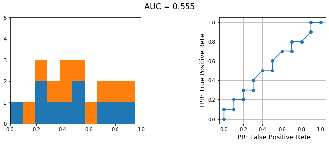
こんなROC曲線になりました。
4. 関数 roc_curve() の返り値について調べてみる
関数roc_curve()の中身を調べてみましょう。
先ほど説明したようなfpr, tpr, thresholds になっていることが分かります。
0番目の thresholds が1.95になっていますが、これは、1番目の閾値に1を加えたもので、fprとtprがともに0となる組みが含まれるように工夫されているようです。
print(fpr.shape, tpr.shape, thres.shape)
ROC_df = pd.DataFrame({'fpr':fpr, 'tpr':tpr, 'thresholds':thres})
ROC_df

最初の例において、引数drop_intermeditateをみてみましょう。
これはデフォルトではFalseになっていますが、TrueにすることでROC曲線の形状に関係しない点は取り除くことができます。
y_pred = [0, 0.15, 0.2, 0.2, 0.25,
          0.3, 0.35, 0.4, 0.4, 0.45,
          0.5, 0.55, 0.55, 0.65, 0.7,
          0.75, 0.8, 0.85, 0.9, 0.95]

y_true = [0, 0, 0, 0, 0,
          0, 0, 0, 0, 0,
          1, 1, 1, 1, 1,
          1, 1, 1, 1, 1]

fpr, tpr, thres = metrics.roc_curve(y_true, y_pred, drop_intermediate =True)
print(fpr.shape, tpr.shape, thres.shape)
(10,) (10,) (10,)
ですので、実際の点の数も減っています。
5. まとめ
今回は機械学習の結果を可視化する際のROC曲線についてまとめてみました。
質問・記事ネタ等募集しています!