0. 最初に
機械学習を用いたデータ分析をしようとする際に、入手したcsvデータからいきなり
「よし!回帰しよう!」
「よし!分類しよう!」
といった風に、いきなりモデル生成に入れることはほとんどありません。むしろ、初心者にはそれまでの壁がなかなか高いです。
ですので、今回はデータの前処理についてまとめてみました。
1. データの読み込み
今回はKaggleのTitanicからデータを借りてきました。
ちなみにjupyterを使ってます。
(jupyterの入出力をQiitaにまとめる方法をご存じの方いらっしゃいましたら教えてください...)
In[1]
%matplotlib inline
import matplotlib as plt
import pandas as pd
import numpy as np
import seaborn as sns
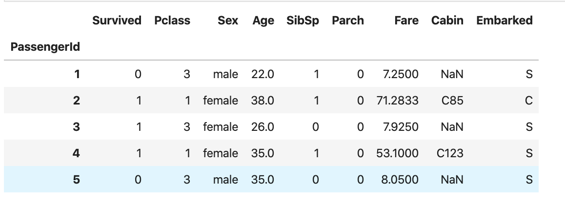
df = pd.read_csv('./train.csv')
df = df.set_index('PassengerId') #一意性がある列をindexに設定する
print(df.shape)
df.head()

2. 分析に不要な列を削除する
In[2]
df = df.drop(['Name', 'Ticket'], axis=1) #分析に不要な列をdropする
df.head()
3. データの型、欠損を確認する
In[3]
print(df.info())
# print(df.dtypes) #データの型のみを確認したければこちら
df.isnull().sum(axis=0)
# df.isnull().any(axis=0) #nullの有無のみを確認する場合はこちら
out[3]
<class 'pandas.core.frame.DataFrame'>
Int64Index: 891 entries, 1 to 891
Data columns (total 9 columns):
Survived    891 non-null int64
Pclass      891 non-null int64
Sex         891 non-null object
Age         714 non-null float64
SibSp       891 non-null int64
Parch       891 non-null int64
Fare        891 non-null float64
Cabin       204 non-null object
Embarked    889 non-null object
dtypes: float64(2), int64(4), object(3)
memory usage: 69.6+ KB
None
Survived      0
Pclass        0
Sex           0
Age         177
SibSp         0
Parch         0
Fare          0
Cabin       687
Embarked      2
dtype: int64
4. 名義尺度の要素の種類をカウント
In[4]
# 名義尺度の要素の種類をカウント
import collections
c = collections.Counter(df['Sex'])
print('Sex:',c)
c = collections.Counter(df['Cabin'])
print('Cabin:',len(c))
c = collections.Counter(df['Embarked'])
print('Embarked:',c)
out[4]
Sex: Counter({'male': 577, 'female': 314})
Cabin: 148
Embarked: Counter({'S': 644, 'C': 168, 'Q': 77, nan: 2})
5. 欠損を削除・補完
In[5]
df = df.drop(['Cabin'], axis=1) #分析には使いにくそうなので削除
df = df.dropna(subset = ['Embarked']) #Cabinは欠損が少ないのでdropnaで行で削除
df = df.fillna(method = 'ffill') #他の列は前のデータから補完
print(df.isnull().any(axis=0))
df.shape
out[5]
Survived    False
Pclass      False
Sex         False
Age         False
SibSp       False
Parch       False
Fare        False
Embarked    False
dtype: bool
(889, 8)
6. ラベルエンコーディング
ラベルエンコーディングを用いてobject(文字)型データをnumerical(数値)型データに変換します。
In[6]
from sklearn.preprocessing import LabelEncoder
for column in ['Sex','Embarked']:
    le = LabelEncoder()
    le.fit(df[column])
    df[column] = le.transform(df[column])
df.head()

SexとEmbarkedに対してラベルエンコーディングがされていることが分かります。
ラベルエンコーディングをしたことで、seabornのpairplotなどを用いてデータの概要を眺めることもできます。
sns.pairplot(df);
連続変数だけを選択して眺めるのも良いと思います。
(下記には厳密には連続変数では無いものも含まれていますが...)
df_continuous = df[['Age','SibSp','Parch','Fare']]
sns.pairplot(df_continuous);

7. ワンホットエンコーディング
ワンホットエンコーディングを用いて数値型にしたデータやその他の名義尺度データをワンホットエンコーディングします。
scikitlearnのOneHotEncoderの上手な使い方が分からなかったのでpandasのget_dummiesを用いました。
In[7]
df = pd.get_dummies(df, columns = ['Pclass','Embarked'])
df.head()
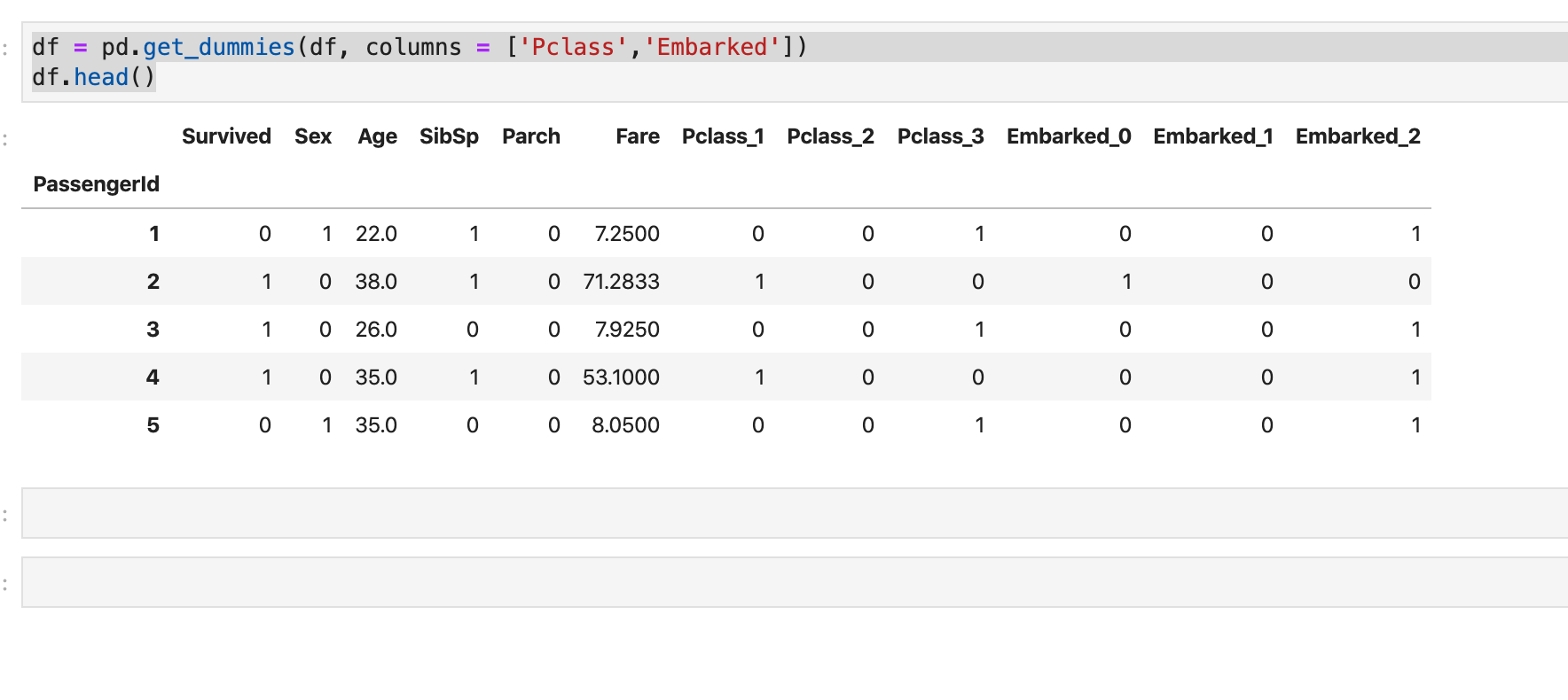
PclassとEmbarkedに対してワンホットエンコーディングがされていることが分かります。
8. まとめ
この流れは多くのデータ分析に共通していると思います。
前処理の流れの参考にしてみて下さい。
コメント、記事ネタなど募集してます。