【Python】飛行機の運動をシミュレートするプログラムをつくる その1「飛行モデルの作成」

はじめに

本プログラムは飛行機の運動がつり合い状態からの微小擾乱と考えた場合の運動をシミュレートするプログラムです。

『航空機力学入門　(加藤寛一郎・大屋昭男・柄沢研治 著　東京大学出版会)』の3章「微小擾乱の運動方程式」をベースに作成しています。

コードを実行すると、こんな感じで飛行機の動きをアニメーション人できます。

プログラムはgooglecolabで実行できるように公開しています。

参考

本プログラムは以下の書籍及びwebサイトを参考になるべく仮定や微小量を消さずに作成しました。

先人たちのおかげでコーディングがとても楽であり、感謝申し上げます。

縦の運動方程式

『航空機力学入門』3.4節
『航空機力学入門』と違い、$M_{\dot{\alpha}}=0$の近似はしておらず式(3.32c)中の$M_{\dot{\alpha}}$を係数とする$\dot{\alpha}$には式(3.32b)を代入

\begin{bmatrix} \dot{u} \\ \dot{\alpha} \\ \dot{q} \\ \dot{\theta} \end{bmatrix}
=\begin{bmatrix}X_{u} & X_{\alpha} & -W_0 & -g\rm{cos}\theta_0 \\
Z_{u}/U_{0} & Z_{\alpha}/U_{0} & 1+Z_{q}/U_{0} & (g/U_0)\rm{sin}\theta_0 \\
M_{u}+M_{\dot{\alpha}}(Z_{u}/U_{0}) & M_{\alpha}+ M_{\dot{\alpha}}(Z_{\alpha}/U_{0}) & M_{q}+M_{\dot{\alpha}}(1+Z_{q}/U_{0}) & (M_{\dot{\alpha}}g/U_0)\rm{sin}\theta_0 \\
0 & 0 & 1 & 0   \end{bmatrix}
\begin{bmatrix} u \\ \alpha \\ q \\ \theta \\ \end{bmatrix}
+\begin{bmatrix}
0 & X_{\delta_{t}} \\
Z_{\delta_{t}}/U_{0} & Z_{\delta_{t}}/U_{0} \\
M_{\delta_{e}}+M_{\dot{\alpha}} (Z_{\delta_{e}}/U_{0}) & M_{\delta_{t}}+M_{\dot{\alpha}} (Z_{\delta_{t}}/U_{0})  \\
0 & 0 \end{bmatrix}
\begin{bmatrix}\delta_e \\ \delta_t \end{bmatrix}

それぞれ説明すると、

縦の状態量
$\mathbf{x}(t)=\begin{bmatrix} u&\alpha& q& \theta \ \end{bmatrix}^{T}$

制御量
$\mathbf{u}(t)=\begin{bmatrix}\delta_e & \delta_t \end{bmatrix}^{T}$

\mathbf{A}=\begin{bmatrix}X_{u} & X_{\alpha} & -W_0 & -g\rm{cos}\theta_0 \\
Z_{u}/U_{0} & Z_{\alpha}/U_{0} & 1+Z_{q}/U_{0} & (g/U_0)\rm{sin}\theta_0 \\
M_{u}+M_{\dot{\alpha}}(Z_{u}/U_{0}) & M_{\alpha}+ M_{\dot{\alpha}}(Z_{\alpha}/U_{0}) & M_{q}+M_{\dot{\alpha}}(1+Z_{q}/U_{0}) & (M_{\dot{\alpha}}g/U_0)\rm{sin}\theta_0 \\
0 & 0 & 1 & 0   \end{bmatrix}

\mathbf{B}=
\begin{bmatrix}
0 & X_{\delta_{t}} \\
Z_{\delta_{t}}/U_{0} & Z_{\delta_{t}}/U_{0} \\
M_{\delta_{e}}+M_{\dot{\alpha}} (Z_{\delta_{e}}/U_{0}) & M_{\delta_{t}}+M_{\dot{\alpha}} (Z_{\delta_{t}}/U_{0})  \\
0 & 0 \end{bmatrix}

微分方程式
$\dot{\mathbf{x}}=\mathbf{A}\mathbf{x}+\mathbf{B}\mathbf{u}$

この微分方程式をルンゲ=クッタ法を用いて数値計算を行う。
scipy.integrate.solve_ivp関数を使用し、RK45、つまり4次精度を保証して5次の項を見て自動で時間幅を調整してくれる関数を使用する。実質matlab等のode45と思われる。

import numpy as np
from scipy.integrate import odeint, solve_ivp
import matplotlib.pyplot as plt


# パラメータ
g=9.81
#初期条件
U0=293.8
W0=0
theta0=0.0

#縦の有次元安定微係数:ロッキードP2V-7
Xu=-0.0215
Zu=-0.227
Mu=0

Xa=14.7
Za=-236
Ma=-3.78
Madot=-0.28

Xq=0
Zq=-5.76
Mq=-0.992

X_deltat=0
Z_deltae=-12.9
Z_deltat=0
M_deltae=-2.48
M_deltat=0



# --- 縦の運動方程式 ---
# 行列A, Bの定義
A_long = np.array([[Xu, Xa, -W0, -g*np.cos(theta0)],
                  [Zu/U0, Za/U0, 1+Zq/U0, (g/U0)*np.sin(theta0)],
                  [Mu+Madot*(Zu/U0), Ma+Madot*(Za/U0), Mq+Madot*(1+Zq/U0), (Madot*g/U0)*np.sin(theta0)],
                  [0, 0, 1, 0]])

B_long = np.array([[0, X_deltat],
                  [Z_deltae/U0, Z_deltat/U0],
                  [M_deltae+Madot*(Z_deltae/U0), M_deltat+Madot*(Z_deltat/U0)],
                  [0, 0]])


# 微分方程式を定義 (solve_ivp用)
def vertical_aircraft_dynamics_ivp(t, x, A_long, B_long, u_long):
  dxdt_long = A_long @ np.atleast_2d(x).T + B_long @ np.atleast_2d(u_long).T
  dxdt_long = dxdt_long.flatten()
  return dxdt_long




# 状態量xの初期値
x0_long = np.array([0, 0, 0, 0])  # 例: 全て0で初期化

# 制御入力u (ここでは定数とする)
u_long = np.array([0.1, 0.2])  # 例: elevator=0.1, throttle=0.2


# 時間ベクトル
t_span = (0, 10)  # 開始時間と終了時間
t_eval = np.linspace(0, 10, 100) # 評価点

# 微分方程式を解く (RK45メソッドを使用)
sol = solve_ivp(vertical_aircraft_dynamics_ivp, t_span, x0_long, args=(A_long, B_long, u_long), method='RK45', t_eval=t_eval)
#print(sol)

# 結果をプロット
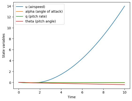
plt.plot(sol.t, sol.y[0], label='u (airspeed)')
plt.plot(sol.t, sol.y[1], label='alpha (angle of attack)')
plt.plot(sol.t, sol.y[2], label='q (pitch rate)')
plt.plot(sol.t, sol.y[3], label='theta (pitch angle)')
plt.legend()
plt.xlabel('Time')
plt.ylabel('State variables')
plt.show()

横・方向の運動方程式

『航空機力学入門』3.4節

情報量
$\mathbf{y}(t)=\begin{bmatrix}\beta & p & r & \phi & \psi \end{bmatrix}^{T}$

制御量
$\mathbf{u}=\begin{bmatrix}\delta_{a} & \delta_{r} \end{bmatrix}^{T}$

\mathbf{A}=\begin{bmatrix}
Y_{\beta}/U_{0} &(W_0+Y_{p})/U_{0} & Y_{r}/U_{0}-1 & g\rm{cos}\theta_0/U_{0} & 0 \\
L'_{\beta} & L'_{p} & L'_{r} & 0 & 0 \\
N'_{\beta} & N'_{p} & N'_{r} & 0 & 0 \\
0 & 1 & \rm{tan}\theta_0 & 0 & 0 \\
0 & 0 & 1/\rm{cos}\theta_0 & 0 & 0
\end{bmatrix}

\mathbf{B}=\begin{bmatrix}
0 & Y_{\delta_{r}}/U_{0} \\
L'_{\delta_{a}} & L'_{\delta_{r}}\\
N'_{\delta_{a}} & N'_{\delta_{r}}\\
0 & 0 \\
0 & 0
\end{bmatrix}

横・方向の運動方程式
$\dot{\mathbf{x}}=\mathbf{A}\mathbf{x}+\mathbf{B}\mathbf{u}$

import numpy as np
from scipy.integrate import odeint, solve_ivp
import matplotlib.pyplot as plt


# パラメータ
g = 9.81
# 初期条件
U0 = 293.8
W0 = 0
theta0 = 0.0

# 横・方向の有次元安定微係数: ロッキードP2V-7
Yb=-45.4
Lb=-1.71
Nb=0.986

Yp=0.716
Lp=-0.962
Np=-0.0632

Yr=2.66
Lr=0.271
Nr=-0.215

#Y_deltaa=0
L_deltaa=1.72
N_deltaa=-0.0436

Y_deltar=9.17
L_deltar=0.244
N_deltar=-0.666






# --- 横・方向の運動方程式 ---
# 行列A, Bの定義
A_lat = np.array([[Yb / U0, (W0 + Yp) / U0, (Yr / U0 - 1), g * np.cos(theta0) / U0, 0],
                  [Lb, Lp, Lr, 0, 0],
                  [Nb, Np, Nr, 0, 0],
                  [0, 1, np.tan(theta0), 0, 0],
                  [0, 0, 1 / np.cos(theta0), 0, 0]])

B_lat = np.array([[0, Y_deltar / U0],
                  [L_deltaa, L_deltar],
                  [N_deltaa, N_deltar],
                  [0, 0],
                  [0, 0]])


# --- 統合モデル ---
def aircraft_dynamics(t, x, A_lat, B_lat, u_lat):

  # 横・方向の運動方程式
  dxdt_lat = A_lat @ np.atleast_2d(x).T + B_lat @ np.atleast_2d(u_lat).T
  dxdt_lat = dxdt_lat.flatten()

  return dxdt_lat

# --- シミュレーション ---

# 初期状態
x0_lat = np.array([0, 0, 0, 0, 0])

# 制御入力
u_lat = np.array([0.05, -0.1])  # 例: aileron=0.05, rudder=-0.1

# 時間ベクトル
t_span = (0, 10)  # 開始時間と終了時間
t_eval = np.linspace(0, 10, 100)  # 評価点

# 微分方程式を解く
sol = solve_ivp(aircraft_dynamics, t_span, x0_lat,
                args=(A_lat, B_lat, u_lat),
                method='RK45', t_eval=t_eval)


# --- 結果のプロット ---
# 横・方向の状態量
plt.figure()
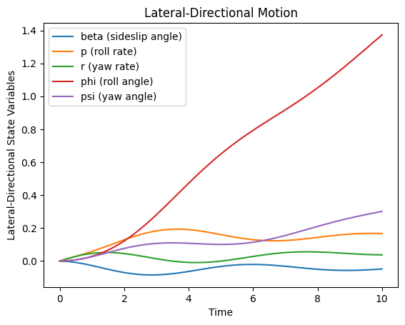
plt.plot(sol.t, sol.y[0], label='beta (sideslip angle)')
plt.plot(sol.t, sol.y[1], label='p (roll rate)')
plt.plot(sol.t, sol.y[2], label='r (yaw rate)')
plt.plot(sol.t, sol.y[3], label='phi (roll angle)')
plt.plot(sol.t, sol.y[4], label='psi (yaw angle)')
plt.legend()
plt.xlabel('Time')
plt.ylabel('Lateral-Directional State Variables')
plt.title('Lateral-Directional Motion')
plt.show()

速度の変換

座標変換

『航空機力学入門』1.5節では、地表座標系から、
Z0軸周りに$\Psi$、
Y1軸周りに$\Theta$、
X2軸周りに$\Phi$だけ回転させて機体座標系に変換している。

わかりやすく説明すると、まずヨー方向に回転させ、次にピッチ、最後にロールをしている。

画像出典：
https://www.sky-engin.jp/blog/eulerian-angles/

Z0軸周りに$\Psi$	Y1軸周りに$\Theta$	X2軸周りに$\Phi$

各軸の回転行列を考えていく。
ここで、回転行列を新たな座標軸にかけると元の座標軸に戻るものとする。

\begin{align}
\mathbf{R}
&=
\underbrace{\begin{bmatrix} \cos{\psi} & -\sin{\psi} & 0 \\ \sin{\psi} & \cos{\psi} & 0 \\ 0 & 0 & 1 \end{bmatrix}}_{z軸周り回転}
\underbrace{\begin{bmatrix} \cos{\theta} & 0 & \sin{\theta} \\ 0 & 1 & 0 \\ -\sin{\theta} & 0 & \cos{\theta} \end{bmatrix}}_{y軸周り回転}
\underbrace{\begin{bmatrix} 1 & 0 & 0 \\ 0 & \cos{\phi} & -\sin{\phi} \\ 0 & \sin{\phi} & \cos{\phi} \end{bmatrix}}_{x軸周り回転} \\
&=
\begin{bmatrix}
c_\psi c_\theta & c_\psi s_\theta s_\phi – c_\phi s_\psi & s_\psi s_\phi + c_\psi c_\phi s_\theta \\
c_\theta s_\psi & c_\psi c_\phi + s_\psi s_\theta s_\phi & c_\phi s_\psi s_\theta – c_\psi s_\phi \\
-s_\theta & c_\theta s_\phi & c_\theta c_\phi
\end{bmatrix}
\end{align}

とすると、機体座標系での位置（添え字b）と全体座標系での位置（添え字e）とすると、以下の関係があり、その時間微分である速度についても同様の関係が成り立つ

\begin{bmatrix} x_e \\ y_e \\ z_e \end{bmatrix}
=
\begin{bmatrix}
c_\psi c_\theta & c_\psi s_\theta s_\phi – c_\phi s_\psi & s_\psi s_\phi + c_\psi c_\phi s_\theta \\
c_\theta s_\psi & c_\psi c_\phi + s_\psi s_\theta s_\phi & c_\phi s_\psi s_\theta – c_\psi s_\phi \\
-s_\theta & c_\theta s_\phi & c_\theta c_\phi
\end{bmatrix}
\begin{bmatrix} x_b \\ y_b \\ z_b \end{bmatrix}

機体座標系

今まで使用してきた運動方程式は任意の機体座標系で使用できるものであった。
『航空機力学入門』1.4節において、機体座標系の取り方は3つ紹介されている。

• 慣性主軸：X軸を機体の慣性主軸に一致することで角運動量の表現が簡単になる
• 安定軸：X軸を定常つり合い飛行時の機体速度ベクトルと一致させる、つまりうだけが速度を持ち、v、wが0
• 機体軸：機体の基準線に一致させる

今回は、飛行経路をプロットする際にコーディングしやすいように機体軸を採用する

各速度の成分は、迎角αと横滑り角βの定義から

$U=U_{0}+u$
$V=V_{c}\sin{\beta}\approx U\sin{\beta}$
$W = U\tan{\alpha}$

縦・横・方向・位置の運動方程式

これまで出てきたものをすべて結合させてシミュレーションを行う

import numpy as np
from scipy.integrate import odeint, solve_ivp
import matplotlib.pyplot as plt
from mpl_toolkits.mplot3d import Axes3D

# --- パラメータ ---
g = 9.81
# 初期条件
U0 = 293.8
W0 = 0
theta0 = 0.0

# 縦の有次元安定微係数: ロッキードP2V-7
Xu = -0.0215
Zu = -0.227
Mu = 0

Xa = 14.7
Za = -236
Ma = -3.78
Madot = -0.28

Xq = 0
Zq = -5.76
Mq = -0.992

X_deltat = 0
Z_deltae = -12.9
Z_deltat = 0
M_deltae = -2.48
M_deltat = 0


# 横・方向の有次元安定微係数: ロッキードP2V-7
Yb=-45.4
Lb=-1.71
Nb=0.986

Yp=0.716
Lp=-0.962
Np=-0.0632

Yr=2.66
Lr=0.271
Nr=-0.215

#Y_deltaa=0
L_deltaa=1.72
N_deltaa=-0.0436

Y_deltar=9.17
L_deltar=0.244
N_deltar=-0.666







# --- 縦の運動方程式 ---
# 行列A, Bの定義
A_long = np.array([[Xu, Xa, -W0, -g * np.cos(theta0)],
                   [Zu / U0, Za / U0, 1 + Zq / U0, (g / U0) * np.sin(theta0)],
                   [Mu + Madot * (Zu / U0), Ma + Madot * (Za / U0), Mq + Madot * (1 + Zq / U0),
                    (Madot * g / U0) * np.sin(theta0)],
                   [0, 0, 1, 0]])

B_long = np.array([[0, X_deltat],
                   [Z_deltae / U0, Z_deltat / U0],
                   [M_deltae + Madot * (Z_deltae / U0), M_deltat + Madot * (Z_deltat / U0)],
                   [0, 0]])


# --- 横・方向の運動方程式 ---
# 行列A, Bの定義
A_lat = np.array([[Yb / U0, (W0 + Yp) / U0, (Yr / U0 - 1), g * np.cos(theta0) / U0, 0],
                  [Lb, Lp, Lr, 0, 0],
                  [Nb, Np, Nr, 0, 0],
                  [0, 1, np.tan(theta0), 0, 0],
                  [0, 0, 1 / np.cos(theta0), 0, 0]])

B_lat = np.array([[0, Y_deltar / U0],
                  [L_deltaa, L_deltar],
                  [N_deltaa, N_deltar],
                  [0, 0],
                  [0, 0]])




# --- 回転行列の定義 ---
def rotation_matrix(psi, theta, phi):
  # z軸周り回転
  R_z = np.array([[np.cos(psi), -np.sin(psi), 0],
                   [np.sin(psi), np.cos(psi), 0],
                   [0, 0, 1]])
  # y軸周り回転
  R_y = np.array([[np.cos(theta), 0, np.sin(theta)],
                   [0, 1, 0],
                   [-np.sin(theta), 0, np.cos(theta)]])
  # x軸周り回転
  R_x = np.array([[1, 0, 0],
                   [0, np.cos(phi), -np.sin(phi)],
                   [0, np.sin(phi), np.cos(phi)]])
  # 全体の回転行列
  R = R_z @ R_y @ R_x
  return R





# --- 統合モデル ---

def aircraft_dynamics(t, x, A_long, B_long, A_lat, B_lat, u_long, u_lat):
  # 縦の運動方程式
  dxdt_long = A_long @ np.atleast_2d(x[:4]).T + B_long @ np.atleast_2d(u_long).T
  dxdt_long = dxdt_long.flatten()

  # 横・方向の運動方程式
  dxdt_lat = A_lat @ np.atleast_2d(x[4:9]).T + B_lat @ np.atleast_2d(u_lat).T
  dxdt_lat = dxdt_lat.flatten()



  # 機体座標系での速度ベクトル
  u_b = U0 + x[0]
  v_b = u_b * np.sin(x[4])
  w_b = u_b * np.tan(x[1])
  vel_b = np.array([u_b, v_b, w_b])

  # 全体座標系での速度ベクトル
  psi = x[8]
  theta = x[3]
  phi = x[7]
  vel_e = rotation_matrix(psi, theta, phi) @ np.atleast_2d(vel_b).T
  vel_e = vel_e.flatten()


  # 縦と横・方向の状態量の変化と位置の変化を結合
  dxdt = np.concatenate((dxdt_long, dxdt_lat, vel_e))
  return dxdt







# --- シミュレーション ---

# 初期状態 (縦と横・方向、位置を結合)
x0_long = np.array([0, 0, 0, 0])  # 例: 全て0で初期化
x0_lat = np.array([0, 0, 0, 0, 0])
x0_pos = np.array([0, 0, 0])
x0 = np.concatenate((x0_long, x0_lat, x0_pos))


# 制御入力 (縦と横・方向)
u_long = np.array([0.01, 0])  # 例: elevator=0.01, throttle=0
u_lat = np.array([0.01, 0])  # 例: aileron=0.01, rudder=-0


# 時間ベクトル
t_span = (0, 200)  # 開始時間と終了時間
t_eval = np.linspace(0, 200, 200)  # 評価点

# 微分方程式を解く (RK45メソッドを使用)
sol = solve_ivp(aircraft_dynamics, t_span, x0,
                args=(A_long, B_long, A_lat, B_lat, u_long, u_lat),
                method='RK45', t_eval=t_eval)






# --- 結果のプロット ---

# 縦の状態量
plt.figure()
plt.plot(sol.t, sol.y[0], label='u (airspeed)')
plt.plot(sol.t, sol.y[1], label='alpha (angle of attack)')
plt.plot(sol.t, sol.y[2], label='q (pitch rate)')
plt.plot(sol.t, sol.y[3], label='theta (pitch angle)')
plt.legend()
plt.xlabel('Time')
plt.ylabel('Longitudinal State Variables')
plt.title('Longitudinal Motion')
plt.show()

# 横・方向の状態量
plt.figure()
plt.plot(sol.t, sol.y[4], label='beta (sideslip angle)')
plt.plot(sol.t, sol.y[5], label='p (roll rate)')
plt.plot(sol.t, sol.y[6], label='r (yaw rate)')
plt.plot(sol.t, sol.y[7], label='phi (roll angle)')
plt.plot(sol.t, sol.y[8], label='psi (yaw angle)')
plt.legend()
plt.xlabel('Time')
plt.ylabel('Lateral-Directional State Variables')
plt.title('Lateral-Directional Motion')
plt.show()

可視化

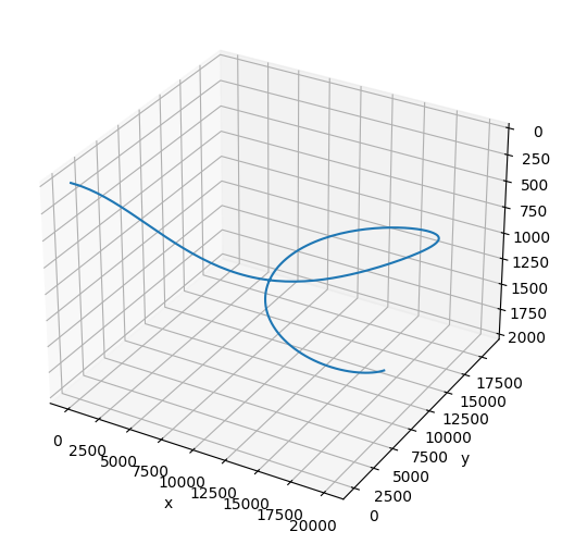
3次元空間上で飛行をプロットする

高さ方向はZ軸負の向きなので描写時には正負を逆にしておく

飛行経路の可視化

# --- 可視化 ---
plt.ion()
fig = plt.figure()
ax = Axes3D(fig)
fig.add_axes(ax)

# 軌跡を描くための全体座標系での座標
x_history = sol.y[9]
y_history = sol.y[10]
z_history = sol.y[11] #Z軸は地面を向いている


# 軌跡をプロット
ax.plot(x_history, y_history, z_history)
ax.set_xlabel("x")
ax.set_ylabel("y")
ax.set_zlabel("z")
# 軸範囲を適切に設定
ax.invert_zaxis()
#ax.set_xlim([-500, 2000])
#ax.set_ylim([-200, 500])
#ax.set_zlim([-500, 200])
#ax.set_zlim(-1000,1000)
plt.show()

飛行のアニメーション

# --- 可視化(アニメーション with 紙飛行機) ---
from IPython.display import HTML
import matplotlib.animation as animation

plt.ion()
fig = plt.figure(dpi=100)
ax = Axes3D(fig)
fig.add_axes(ax)


def update(i):
    ax.clear()
    ax.plot(x_history[:i+1], y_history[:i+1], z_history[:i+1])


    # 軌跡をプロット
    ax.set_xlabel("x")
    ax.set_ylabel("y")
    ax.set_zlabel("z")
    # 軸範囲を適切に設定
    ax.set_xlim(min(x_history),max(x_history))
    ax.set_ylim(min(y_history),max(y_history))
    ax.invert_zaxis()
    ax.set_zlim((max(z_history),min(z_history)))

anim = animation.FuncAnimation(fig, update, frames=range(0, len(sol.t), 10), interval=100)
anim.save("flight_path.gif", writer="imagemagick")
HTML(anim.to_jshtml())

紙飛行機を追加した飛行経路

飛行機の翼端灯に習い、右を緑、左を赤色に塗った紙飛行機を追加する。

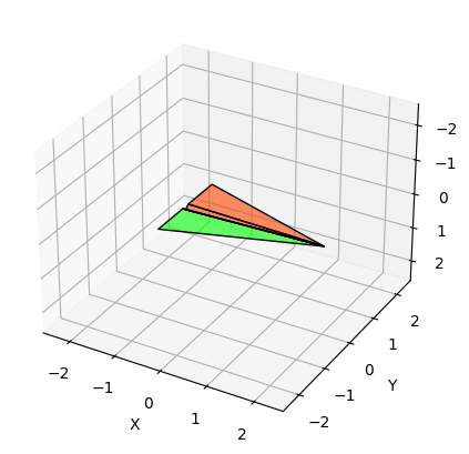
さらに、高度の変化がわかりやすいように垂線を赤色で示す

import matplotlib.pyplot as plt
from mpl_toolkits.mplot3d import Axes3D
import numpy as np
import mpl_toolkits.mplot3d.art3d as art3d


def plot_paper_airplane(x, y, z, phi, theta, psi, scale, ax):
    """
    3次元座標と角度が与えられたとき、その状態の紙飛行機のような図形をプロットする

    Args:
      x: x座標
      y: y座標
      z: z座標
      psi: ロール角 (ラジアン)
      theta : ピッチ角 (ラジアン)
      phi: ヨー角 (ラジアン)
      機体の大きさをいじりたければscaleを変える

    """

    #三角形を描く
    poly_left_wing = scale * np.array([[2, 0.0, 0],
                                      [-1, 1, 0],
                                      [-1, 0.1, 0]])
    poly_right_wing = poly_left_wing.copy()
    poly_right_wing[:,1] = -1 * poly_right_wing[:,1]

    poly_left_body = scale * np.array([[2, 0.0, 0.0],
                                      [-1, 0.0, +0.1],
                                      [-1, 0.1, 0.0]])
    poly_right_body = poly_left_body.copy()
    poly_right_body[:,1] = -1 * poly_right_body[:,1]



    R = rotation_matrix(psi, theta, phi) # yaw, pitch, roll


    for points in [poly_left_wing, poly_left_body, ]:
        # 紙飛行機の点を回転
        translated_rotated_points = (R @ points.T).T + np.array([x, y, z])
        #描写
        ax.add_collection3d(art3d.Poly3DCollection([translated_rotated_points],facecolors='orangered', linewidths=1, edgecolors='k', alpha=0.6))

    for points in [poly_right_wing, poly_right_body]:
        # 紙飛行機の点を回転
        translated_rotated_points = (R @ points.T).T + np.array([x, y, z])
        #描写
        ax.add_collection3d(art3d.Poly3DCollection([translated_rotated_points],facecolors='lime', linewidths=1, edgecolors='k', alpha=0.6))


## 紙飛行機単体のプロット
#fig = plt.figure(figsize=(5,5))
#ax = fig.add_subplot(111, projection='3d')#,aspect='equal')
#plot_paper_airplane(x=0, y=0, z=0, phi=0, theta=0, psi=0, scale=1, ax=ax)
#ax.set_xlabel('X')
#ax.set_ylabel('Y')
#ax.set_zlabel('Z')
#ax.invert_zaxis()
#ax.set_xlim(-2.5, 2.5)
#ax.set_ylim(-2.5, 2.5)
#ax.set_zlim(2.5, -2.5, )
#plt.show()



# --- 可視化(アニメーション with 紙飛行機) ---
from IPython.display import HTML
import matplotlib.animation as animation

plt.ion()
fig = plt.figure(dpi=100)
ax = Axes3D(fig)
fig.add_axes(ax)


def update(i):
    ax.clear()
    ax.plot(x_history[:i+1], y_history[:i+1], z_history[:i+1])

    #紙飛行機
    plot_paper_airplane(x=x_history[i],  y=y_history[i], z=z_history[i], phi=sol.y[7][i], theta=sol.y[3][i], psi=sol.y[8][i], scale=1000, ax=ax)
    #垂線
    ax.add_line(art3d.Line3D([x_history[i],x_history[i]],[y_history[i],y_history[i]],[z_history[i],max(z_history)], color='r'))



    # 軌跡をプロット
    ax.set_xlabel("x")
    ax.set_ylabel("y")
    ax.set_zlabel("z")
    # 軸範囲を適切に設定
    ax.set_xlim(min(x_history),max(x_history))
    ax.set_ylim(min(y_history),max(y_history))
    ax.invert_zaxis()
    ax.set_zlim((max(z_history),min(z_history)))

anim = animation.FuncAnimation(fig, update, frames=range(0, len(sol.t), 5), interval=100)
anim.save("paper_plane.gif", writer="imagemagick")
HTML(anim.to_jshtml())

最後に

今回は飛行機の運動をシミュレーションするプログラムを作りました。
はじめは教科書を読んでいるだけではちんぷんかんぷんだったのですが、
実際にプログラムを作ってみると式の意味が理解できたり、Pythonでの数値解析の方法が学べたりととてもいい経験になりました。

今回は「その1」だったのですが、
その2では、リアルタイムに入力を受け付けられるようにします。

その3でDQNで飛行制御できたりできないかなーと考えています。