環境設定
pyenv install anaconda3-2.1.0
{~/.bash_profileに追加する設定}
eval "$(pyenv init -)"
# python3のanaconda利用
pyenv global anaconda3-2.1.0
# 元に戻る場合
pyenv global system
jupyter(ipython notebookの基本的な使い方)
1行実行
Ctrl + Enter
新しい行を作って実行
Shift + Enter
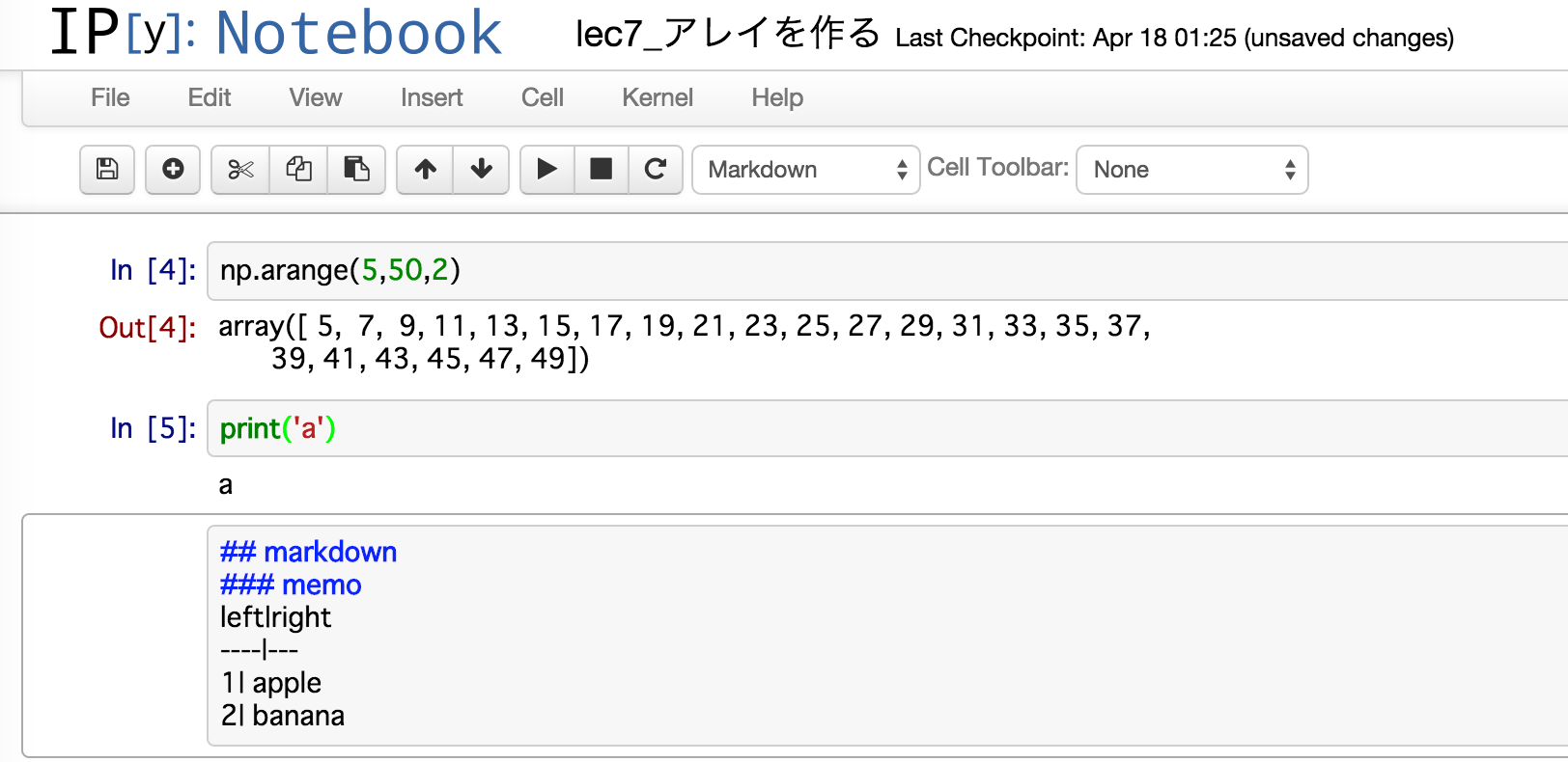
markdownでメモ作成
helpの下でMarkdownを選択すれば、markdownを利用できる。
Section2
Lesson4
ipython notebookの使い方
適当なディレクトリでipython notebookを実行すると、ブラウザでipythonの画面が立ち上がる。
作業ディレクトリは:/usr/local/wk/udemy_lecture
Section3
Lecture7
numpyのarrayを使う。
一番簡単なのは、リストから作る。
my_list1 = [1, 2, 3, 4]
my_array1 = np.array(my_list1)
my_array1
array([1, 2, 3, 4])
リスト同士をくっつけて、多次元配列にできる
my_list2 = [11, 22, 33, 44]
my_lists = [my_list1, my_list2]
my_lists
[[1, 2, 3, 4], [11, 22, 33, 44]]
my_array2 = np.array(my_lists)
my_array2
array([[ 1,  2,  3,  4],
       [11, 22, 33, 44]])
他にも
# 行列数確認
my_array2.shape
(2, 4)

# 0行列の作成
my_zeros = np.zeros(5)
# データタイプの確認(np.arrayは全要素が同じデータタイプじゃなきゃだめ)
my_zeros.dtype
dtype('float64')
# 全要素が1の行列作成
np.ones((5, 5))

array([[ 1.,  1.,  1.,  1.,  1.],
       [ 1.,  1.,  1.,  1.,  1.],
       [ 1.,  1.,  1.,  1.,  1.],
       [ 1.,  1.,  1.,  1.,  1.],
       [ 1.,  1.,  1.,  1.,  1.]
       ])
# 単位行列作成
np.eye(5)
array([[ 1.,  0.,  0.,  0.,  0.],
       [ 0.,  1.,  0.,  0.,  0.],
       [ 0.,  0.,  1.,  0.,  0.],
       [ 0.,  0.,  0.,  1.,  0.],
       [ 0.,  0.,  0.,  0.,  1.]])
# 連番の行列作成
np.arange(5)
array([0, 1, 2, 3, 4])
# その他
array([0, 1, 2, 3, 4])
array([ 5,  7,  9, 11, 13, 15, 17, 19, 21, 23, 25, 27, 29, 31, 33, 35, 37,
       39, 41, 43, 45, 47, 49])
Lecture8
arrayの使い方(基本)
arr1= np.array([[1, 2, 3, 4],[8, 9, 10, 11]])
arr1 * arr1
array([[  1,   4,   9,  16],
       [ 64,  81, 100, 121]])
arr1 - arr1
array([[0, 0, 0, 0],
       [0, 0, 0, 0]])
1 / arr1
array([[ 1.        ,  0.5       ,  0.33333333,  0.25      ],
       [ 0.125     ,  0.11111111,  0.1       ,  0.09090909]])
# 3乗
arr1 ** 3
array([[   1,    8,   27,   64],
       [ 512,  729, 1000, 1331]])
Lecture9
添え字
import numpy as np
import numpy as np
arr
array([ 0,  1,  2,  3,  4,  5,  6,  7,  8,  9, 10])
arr[8]
8
# スライス
arr[1:5]
array([1, 2, 3, 4])
arr[0:5] = 100
array([100, 100, 100, 100, 100,   5,   6,   7,   8,   9,  10])
arr = np.arange(0,11)
# スライス表現を使って、コピーしたアレイを変更するときは注意!
slice_arr = arr[0:6]
slice_arr
array([0, 1, 2, 3, 4, 5])
slice_arr[:] = 99
slice_arr
array([99, 99, 99, 99, 99, 99])
arr
array([99, 99, 99, 99, 99, 99,  6,  7,  8,  9, 10])
# やるなら、コピーして行列を新たに作る。
arr_copy = arr.copy()
arr_copy
array([99, 99, 99, 99, 99, 99,  6,  7,  8,  9, 10])
arr_copy[:] = 50
arr
array([99, 99, 99, 99, 99, 99,  6,  7,  8,  9, 10])

arr_2d = np.array([[5, 10, 15],[20, 25,30],[35,40,45]])
arr_2d
array([[ 5, 10, 15],
       [20, 25, 30],
       [35, 40, 45]])
arr_2d[1]
array([20, 25, 30])
arr_2d[1][0]
20
arr_2d[1, 0]
20

arr_2d[0,1:2]
array([[10, 15],
       [25, 30]])
arr_2d = np.zeros((10,10))
arr_2d
array([[ 0.,  0.,  0.,  0.,  0.,  0.,  0.,  0.,  0.,  0.],
       [ 0.,  0.,  0.,  0.,  0.,  0.,  0.,  0.,  0.,  0.],
       [ 0.,  0.,  0.,  0.,  0.,  0.,  0.,  0.,  0.,  0.],
       [ 0.,  0.,  0.,  0.,  0.,  0.,  0.,  0.,  0.,  0.],
       [ 0.,  0.,  0.,  0.,  0.,  0.,  0.,  0.,  0.,  0.],
       [ 0.,  0.,  0.,  0.,  0.,  0.,  0.,  0.,  0.,  0.],
       [ 0.,  0.,  0.,  0.,  0.,  0.,  0.,  0.,  0.,  0.],
       [ 0.,  0.,  0.,  0.,  0.,  0.,  0.,  0.,  0.,  0.],
       [ 0.,  0.,  0.,  0.,  0.,  0.,  0.,  0.,  0.,  0.],
       [ 0.,  0.,  0.,  0.,  0.,  0.,  0.,  0.,  0.,  0.]])

arr_length = arr_2d.shape[1]
arr_length
10

for i in range(arr_length):
    arr_2d[i] = i

arr_2d
array([[ 0.,  0.,  0.,  0.,  0.,  0.,  0.,  0.,  0.,  0.],
       [ 1.,  1.,  1.,  1.,  1.,  1.,  1.,  1.,  1.,  1.],
       [ 2.,  2.,  2.,  2.,  2.,  2.,  2.,  2.,  2.,  2.],
       [ 3.,  3.,  3.,  3.,  3.,  3.,  3.,  3.,  3.,  3.],
       [ 4.,  4.,  4.,  4.,  4.,  4.,  4.,  4.,  4.,  4.],
       [ 5.,  5.,  5.,  5.,  5.,  5.,  5.,  5.,  5.,  5.],
       [ 6.,  6.,  6.,  6.,  6.,  6.,  6.,  6.,  6.,  6.],
       [ 7.,  7.,  7.,  7.,  7.,  7.,  7.,  7.,  7.,  7.],
       [ 8.,  8.,  8.,  8.,  8.,  8.,  8.,  8.,  8.,  8.],
       [ 9.,  9.,  9.,  9.,  9.,  9.,  9.,  9.,  9.,  9.]])

arr_2d[[2,4,6,8]]
array([[ 2.,  2.,  2.,  2.,  2.,  2.,  2.,  2.,  2.,  2.],
       [ 4.,  4.,  4.,  4.,  4.,  4.,  4.,  4.,  4.,  4.],
       [ 6.,  6.,  6.,  6.,  6.,  6.,  6.,  6.,  6.,  6.],
       [ 8.,  8.,  8.,  8.,  8.,  8.,  8.,  8.,  8.,  8.]])

arr_2d[[6,4,2,7]]
array([[ 6.,  6.,  6.,  6.,  6.,  6.,  6.,  6.,  6.,  6.],
       [ 4.,  4.,  4.,  4.,  4.,  4.,  4.,  4.,  4.,  4.],
       [ 2.,  2.,  2.,  2.,  2.,  2.,  2.,  2.,  2.,  2.],
       [ 7.,  7.,  7.,  7.,  7.,  7.,  7.,  7.,  7.,  7.]])
lecture10
行列の入れ替え
import numpy as np
# 0~8を3行3列の行列で作成
arr = np.arange(9).reshape((3,3))
arr
array([[0, 1, 2],
       [3, 4, 5],
       [6, 7, 8]])
# 転置
arr.T
array([[0, 3, 6],
       [1, 4, 7],
       [2, 5, 8]])

arr.transpose()
array([[0, 3, 6],
       [1, 4, 7],
       [2, 5, 8]])

# 内積計算
np.dot(arr.T,arr)
array([[45, 54, 63],
       [54, 66, 78],
       [63, 78, 93]])

arr3d = np.arange(12).reshape(3,2,2)
arr3d
array([[[ 0,  1],
        [ 2,  3]],

       [[ 4,  5],
        [ 6,  7]],

       [[ 8,  9],
        [10, 11]]])
lecture11
arrayの計算用関数
import numpy as np
arr = np.arange(11)
arr
array([ 0,  1,  2,  3,  4,  5,  6,  7,  8,  9, 10])
# ルート
np.sqrt(arr)
array([ 0.        ,  1.        ,  1.41421356,  1.73205081,  2.        ,
        2.23606798,  2.44948974,  2.64575131,  2.82842712,  3.        ,
        3.16227766])
# exp
np.exp(arr)
array([  1.00000000e+00,   2.71828183e+00,   7.38905610e+00,
         2.00855369e+01,   5.45981500e+01,   1.48413159e+02,
         4.03428793e+02,   1.09663316e+03,   2.98095799e+03,
         8.10308393e+03,   2.20264658e+04])
# 標準正規分布に従う乱数発生
A = np.random.randn(10)
A
array([-0.23874366, -0.29824394, -1.53125686, -1.294902  ,  1.05791343,
        0.27597892,  1.04747699, -0.00482985,  1.04880337, -0.11188837])

B = np.random.randn(10)
B
array([-0.41609336, -1.58252599, -0.83023645,  0.83826666, -0.1137154 ,
        1.22981003,  0.45385263, -1.1296005 ,  0.80177283,  1.35417939])

np.add(A, B)
array([-0.65483702, -1.88076993, -2.36149331, -0.45663534,  0.94419803,
        1.50578895,  1.50132962, -1.13443035,  1.8505762 ,  1.24229102])

# 大きい方を取得
np.maximum(A, B)
array([-0.23874366, -0.29824394, -0.83023645,  0.83826666,  1.05791343,
        1.22981003,  1.04747699, -0.00482985,  1.04880337,  1.35417939])
lecture13
以下参照。。
/usr/local/wk/udemy_lecture/lec12_アレイを使ったデータ処理.ipynb
lecture39(ビニング)
簡単なgroup by みたいなことができる。
{binning.py}
import pandas as pd
# 集計対象のリスト
years = [1990, 1991, 1992, 2008, 2012, 2015, 1987, 1969, 2013, 2008, 1999]
# 集計単位のリスト
decade_bins = [1960, 1970, 1980, 1990, 2000, 2010, 2020]
# 集計対象を、集計単位でカット。
decade_cat = pd.cut(years,decade_bins)
pd.value_counts(decade_cat)
>(2010, 2020]    3
>(1990, 2000]    3
>(1980, 1990]    2
>(2000, 2010]    2
>(1960, 1970]    1
>dtype: int64
lecture42(データをまとめるGroupBy)
pandasのDataFrameでGroupByを実行
{groupby.py}
import numpy as np
import pandas as pd
from pandas import DataFrame
# テスト用データ作成
dframe = DataFrame({'k1' : ['X', 'X', 'Y', 'Y', 'Z'],
                    'k2' : ['alpha', 'beta', 'alpha', 'beta', 'alpha'],
                    'dataset1' : np.random.randn(5),
                    'dataset2' : np.random.randn(5)})

dframe
>dataset1	dataset2	k1	k2
>0	1.481754	0.618496	X	alpha
>1	1.155727	0.194219	X	beta
>2	0.926681	1.075756	Y	alpha
>3	1.152604	0.856419	Y	beta
>4	0.289140	0.617901	Z	alpha

# dataset1に対し、k1をキーにgroupby実行
group1 = dframe['dataset1'].groupby(dframe['k1'])
# 平均を取得
group1.mean()
>k1
>X     1.318740
>Y     1.039643
>Z     0.289140
>Name: dataset1, dtype: float64

# シンプルにk1で平均を取得
dframe.groupby('k1').mean()
>	dataset1	dataset2
>k1
>X	1.318740	0.406357
>Y	1.039643	0.966087
>Z	0.289140	0.617901

# 属するデータの個数を調べる
dframe.groupby(['k1']).size()
>k1
>X     2
>Y     2
>Z     1
>dtype: int64

# groupbtyした結果をそのままみる
for name, group in dframe.groupby('k1'):
    print('This is the {} group'.format(name))
    print(group)
    print('\n')

>This is the X group
>   dataset1  dataset2 k1     k2
>0  1.481754  0.618496  X  alpha
>1  1.155727  0.194219  X   beta

>This is the Y group
>   dataset1  dataset2 k1     k2
>2  0.926681  1.075756  Y  alpha
>3  1.152604  0.856419  Y   beta

>This is the Z group
>   dataset1  dataset2 k1     k2
>4   0.28914  0.617901  Z  alpha
lecture46(クロス集計表)
クロス集計表作る。
{crosstab.py}
import pandas as pd
from io import StringIO

data = '''Sample  Animal  Intelligence
1 Dog Dumb
2 Dog Dumb
3 Cat Smart
4 Cat Smart
5 Dog Smart
6 Cat Smart'''

dframe = pd.read_table(StringIO(data), sep='\s+')
# クロス集計実行(animalとIntelligenceでクロス集計)
pd.crosstab(dframe.Animal, dframe.Intelligence, margins = True)

>Intelligence	Dumb	Smart	All
>Animal
>Cat	0	3	3
>Dog	2	1	3
>All	2	4	6