More than 1 year has passed since last update.

PyTorch備忘録3

PyTorch

Last updated at 2024-03-02Posted at 2024-03-02

過去学習分
- PyTorch基礎 : https://qiita.com/yooooshiii/items/dc281e8d70caf4b0d084
- PyTorch Lightningの利用：https://qiita.com/yooooshiii/items/b18b09381453c7bf657c

PyTorchによるtime series forecsting

Deep Learning利用時の注意点

各特徴量のスケーリング必要
- すべての特徴量を平均０、分散１に標準化することで、勾配を求めやすくする
不要な特徴量の削除
- Machine Learningでは、不要な（役に立たない）特徴量が入っていても、予測に大きな影響を与えないケースが多いが、Deep Learningにおいては、不要な特徴量から変な学習をする可能性があるため、役に立ってない特徴量は削除した方が良い
カテゴリカル変数の変換
- one-hot-encodingをすると、0ばかりのスパースデータになってしまい、学習がうまくいかなくなる。また、one-hotだと週末（土日）と平日の違いなどを表現できない。そこで、Embedding vectorsの利用などがお勧め。　実装は、nn.Embeddingを用いてEmbedding層を追加する。
グローバルモデリングで、複数の時系列データの中でマジョリティを占める特徴を持つ時系列だけからしか学習しない場合の対応
- batchサンプリング時に、満遍なく様々な時系列が選ばれるようにするために、detaloader()クラスはWeightedRandomSamplerを持つので、これをsamplerに入れる

Pytorchにおける時系列データ用dataset

Pytorch_forecasting.data.timeseries.TiseseriesDataset クラス
Pytorchで時系列データを扱うためのクラス、以下の事を自動で行ってくれる
- 変数のスケーリングとエンコーディング
- 目的変数の標準化
- Pandas Dataframeから torch tensor への変換
- 未来における既知および未知の静的・動的変数に関する情報の保持
- 祝日など関連カテゴリ情報の保持
- 時系列データのダウンサンプリング
- train, validation, testの各データの生成
バッチ処理用には、to_dataloade()メソッドを用いて、DataSetクラスからdataloaderクラスに変換する

TimeSeriesDataSetにおける、重要なパラメータ

min/max encorder length
- the minimum and maximum length for encoding or the history length, for example if there are 20 time steps in total and we want a min_encoder_length=3 and max_encoder_length=8, then several sequences will be generated which are at leastof length min_encoder_length and at most of length max_encoder_length and generally as large history as possible will be used. The advantage of this flexibility in the length is : If your dataset has also very short time series to predict, this flexibility ensures you can make predictions for these as well while using more history for longer time series.
min/max prediction length
- minimum / maximum prediction / decorder length
group ids
- list of column names identifying a time series. This means that the group_idx identify a sample together with the time_idx. If you have only one timeseris, set this to the name of column that is constant.
target_normalizer
- This takes in a transformer that normalizes the targets. There are a few normalizers built into Pytorch Forecasting - TorchNormalizer, GroupNormalizer, EncoderNormalizer.
- TorchNormalizer
  - This does standard and robust scaling of the targets as a whole, whereas GroupNormalizer does the same but with each group separately(a group is difined by group_idx).
- EncoderNormalizer does the scaling at runtime by normalizing using the values in each window.
categorical_encoders
- This parameter takes in a dictionary of scikit-learn transformers as a category encoder. By default, the category encoding is similar to LabelEncoder, which replaces each unique categorical values with a number, adding as additional category for unknown and NaN values.

Deep Learningにおける時系列予測の主要モデル

N-Beats
- トレンドを多項式回帰で、季節性をフーリエ変換を用いて予測する
- 上記の理由より、モデルに説明能力がある
- 外部説明変数を利用できない
N-HiTS
- N-Beatsの改良版
- 計算コストが従来のDeepLearningモデルよりも低くなっている
- N-Beatsにあったinterpretable blockが無くなったので、説明力がない
TFT(Temporal Fusion Transformer)
- Transformerを用いたモデル
- Transformerのinput-embedding(単語のベクトル変換)をinput-featureに変えた事で外部特徴量を追加できる
- Attentionメカニズムにより長期記憶を保存できる
- この長期記憶の保持によりコンテキストを学習でき、このコンテキストが時系列でのトレンドや周期性の把握に使われている
- Varaiable Selection Networkにより変数選択が行われる
- 特徴量重要度の確認が可能

PyTorch Forecastingの作成手順

TimeseriesDatasetを用いてtraining datasetを作成
from_dataset()メソッドによりtraining datasetからvalidation datasetを作成し、同時にtest datasetを作成
from_dataset()メソッドによりモデルをインスタンス化
lightning.Trainer()オブジェクトを作成
５. tuner.lr_find()メソッドで最適なlearning rateを見つける
early stoppingを利用してモデルを学習し、accuracyなどの学習状況はtensorboardで確認する
optunaなどでハイパーパラメータのチューニングを行う

TFTコード例

以下のTFT利用紹介サイトを用いて学習
- https://pytorch-forecasting.readthedocs.io/en/latest/tutorials/stallion.html

1. Data Preprocessing

利用データセット(電力量)のダウンロード

wget https://archive.ics.uci.edu/ml/machine-learning-databases/00321/LD2011_2014.txt.zip

ライブラリ(その他必要なものは都度入れている)

import numpy as np
import pandas as pd
from pytorch_forecasting import TimeSeriesDataSet

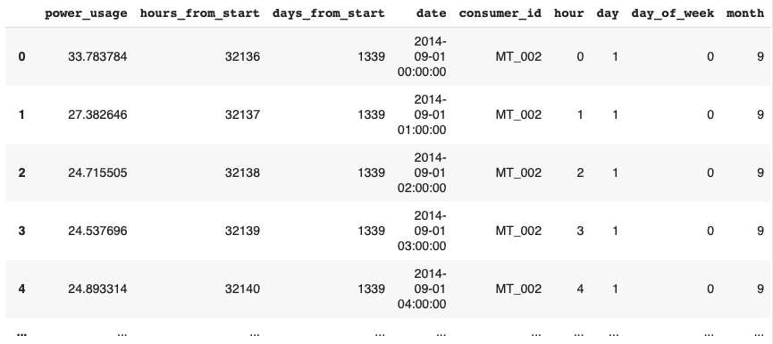
データの中身

data = pd.read_csv('/content/drive/MyDrive/LD2011_2014.txt', index_col=0, sep=';', decimal=',')
data.index = pd.to_datetime(data.index)
data.sort_index(inplace=True)
data.head()

MT_*が各家庭を表す
各家庭の電力使用量を予測する
以下、MT_002, 004, 005, 006, 008の電力を予測する

# aggregate to hourly data
# We train our model on 5 consumers only ( for those with non-zero values)

data = data.resample('1h').mean().replace(0., np.nan)
earliest_time = data.index.min()
df = data[['MT_002', 'MT_004', 'MT_005', 'MT_006', 'MT_008']]

Now, we prepare our dataset for the TimeSeriesDataset format. Notice that each column represents a different time-series. Hence, We 'melt' our dataframe, so that time-series are stacked vertically instead of horizontally. In the process, we create our nuew features.

df_list = []

for label in df: # dfだけで、列名がループされる
  # 列ごとに処理
  ts = df[label]
  start_date = min(ts.fillna(method='ffill').dropna().index)
  end_date = max(ts.fillna(method='bfill').dropna().index)

  active_range = (ts.index >= start_date) & (ts.index <= end_date)
  ts = ts[active_range].fillna(0.) # 対象期間のNoneを0で置き換えたSeries

  tmp = pd.DataFrame({'power_usage': ts})
  date = tmp.index
  # time indexの作成 (8760, 8761,.....)
  tmp['hours_from_start'] = (date - earliest_time).seconds /60/60 + (date - earliest_time).days * 24
  tmp['hours_from_start'] = tmp['hours_from_start'].astype('int')
  # 新しい変数列作成
  tmp['days_from_start'] = (date - earliest_time).days
  tmp['date'] = date
  tmp['consumer_id'] = label
  tmp['hour'] = date.hour
  tmp['day'] = date.day
  tmp['day_of_week'] = date.dayofweek
  tmp['month'] = date.month

  # stack all time series vertically
  df_list.append(tmp)

  # stack結果をdf化
time_df = pd.concat(df_list).reset_index(drop=True)

# match results in the original paper
time_df = time_df[(time_df['days_from_start'] >= 1096) & (time_df['days_from_start'] < 1346)].copy()
time_df

time_dfの中身
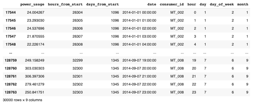
"hours_from_start" variable will be the time index

2. Create DataLoders

Our model uses a lookback window of one week (7*24) to predict the power usage of the next 24 hours.

# from pytorch_forecasting.models.base_model import GroupNormalizer
from pytorch_forecasting.data import GroupNormalizer

max_prediction_length = 24 # 24時間分の電気利用量を予測
max_encoder_length = 7 * 24 # 過去1週間をエンコーダーの長さに指定
# train_cutoffは何に使う -> 予測時に必要なエンコーダデータをトレインから取り出している。（validationデータに付与するため！！！）
train_cutoff = time_df['hours_from_start'].max() - max_prediction_length

training = TimeSeriesDataSet(
    time_df[lambda x: x.hours_from_start <= train_cutoff], # "hours_from_start"列の値が train_cutoff以下のレコードを学習に利用
    time_idx= 'hours_from_start',
    target= 'power_usage',
    group_ids= ['consumer_id'],
    min_encoder_length= max_encoder_length // 2,
    max_encoder_length= max_encoder_length,
    min_prediction_length= 1,
    max_prediction_length= max_prediction_length,
    static_categoricals= ['consumer_id'],
    time_varying_known_reals= ['hours_from_start', 'day', 'day_of_week', 'month', 'hour'],
    time_varying_unknown_reals= ['power_usage'],
    target_normalizer= GroupNormalizer(
        groups= ['consumer_id'], transformation='softplus'
    ), # normalize by group
    add_relative_time_idx= True,
    add_target_scales= True,
    add_encoder_length= True
)

validation = TimeSeriesDataSet.from_dataset(training, time_df, predict=True, stop_randomization=True)

# create dataloaders for our model
batch_size = 94
# if you have a strong GPU, feel free to increase the number of workers
train_dataloader = training.to_dataloader(train=True, batch_size=batch_size, num_workers=0)
val_dataloader = validation.to_dataloader(train=False, batch_size=batch_size * 10, num_workers=0)

3. Baseline Model

As a naive baseline, we predict the power usage curve of the previous day

import torch
from pytorch_forecasting.models.baseline import Baseline

actuals = torch.cat([y for x, (y, weight) in iter(val_dataloader)]).to('cuda')
baseline_predictions = Baseline().predict(val_dataloader)
(actuals - baseline_predictions).abs().mean().item()
# 上記ベースモデルの誤差 -> 25.139617919921875

baseline_predictions
# ベースモデルの予測値
tensor([[263.4680, 263.4680, 263.4680, 263.4680, 263.4680, 263.4680, 263.4680,
         263.4680, 263.4680, 263.4680, 263.4680, 263.4680, 263.4680, 263.4680,
         263.4680, 263.4680, 263.4680, 263.4680, 263.4680, 263.4680, 263.4680,
         263.4680, 263.4680, 263.4680]], device='cuda:0')

4. Training the Temporal Fusion Transformer Model

Notice the following things:
- We use the EarlyStopping callback to monitor the validation loss.
- We use Tensorboard to log our training and validation metrics.
- Our model uses Quntile Loss - a special type of loss that helps us output the prediction intervals.
- We use 4 attention heads, like the original paper.

from lightning.pytorch.callbacks.early_stopping import EarlyStopping
from lightning.pytorch.callbacks.lr_monitor import LearningRateMonitor
from lightning.pytorch.loggers.tensorboard import TensorBoardLogger

# import pytorch_lightning as pl
import lightning.pytorch as pl

from pytorch_forecasting.models import TemporalFusionTransformer
from pytorch_forecasting.models.temporal_fusion_transformer import QuantileLoss

early_stop_callback = EarlyStopping(monitor= 'val_loss', min_delta= 1e-4, patience= 5, verbose= True, mode= 'min')
lr_logger = LearningRateMonitor()
logger = TensorBoardLogger('lightning_logs')

trainer = pl.Trainer(
    max_epochs= 45,
    accelerator= 'gpu',
    devices= 1,
    enable_model_summary= True,
    gradient_clip_val= 0.1,
    callbacks= [lr_logger, early_stop_callback],
    logger= logger
)

tft = TemporalFusionTransformer.from_dataset(
    training,
    learning_rate= 0.001,
    hidden_size= 160,
    attention_head_size= 4,
    dropout = 0.1,
    hidden_continuous_size= 160,
    output_size= 7, # there are 7 quantiles by default: [0.02, 0.1, 0.25, 0.5, 0.75, 0.9, 0.98]
    loss= QuantileLoss(),
    log_interval= 10,
    reduce_on_plateau_patience= 4
)

trainer.fit(
    tft,
    train_dataloaders= train_dataloader,
    val_dataloaders= val_dataloader
)

# ベストモデルでモデル作成
best_model_path = trainer.checkpoint_callback.best_model_path
best_tft = TemporalFusionTransformer.load_from_checkpoint(best_model_path)

5. Check Tensorboad

省略

6. Model Evaluation

Get predictions on the validation set and calculate the average P50(quntile median)loss

actuals = torch.cat([y[0] for x, y in iter(val_dataloader)]).to('cuda')
predictions = best_tft.predict(val_dataloader) # <- 引数なしで予測すると、quantileの中央値が返ってくるっぽい！！！

# 予測結果
predictions
'''
tensor([[ 30.8523,  28.2646,  26.5734,  25.8994,  26.1087,  27.5221,  29.7394,
          30.4027,  30.8232,  31.9222,  34.2415,  36.0092,  34.2732,  33.0783,
          31.5995,  30.3648,  30.1025,  30.3497,  31.8759,  35.5061,  36.4556,
          33.2728,  32.6338,  31.2231],
        [122.2819, 108.7793,  98.5338,  94.7915,  96.0896,  95.7922,  87.6682,
          72.3900,  84.2571,  95.6275, 116.5361, 136.3063, 136.4577, 108.7987,
          98.5752,  93.1882,  89.1331,  87.4842,  92.5298, 108.9735, 122.7908,
         151.0728, 147.6250, 131.7474],
        [ 44.4004,  40.9469, ...

predictions.shape
# -> torch.Size([5, 24])

# average p50 loss overall
print((actuals - predictions).abs().mean().item())
-> 6.424372673034668

# average p50 loss per time series
print((actuals - predictions).abs().mean(axis=1))
-> tensor([ 0.8487,  7.5022,  2.3923,  9.1828, 12.1958], device='cuda:0')

7. Plot Predictions For A Specifit Time Series

If we pass the mode=raw on the predict() method, we get more information, including predictions for all seven quantiles. We also have access to the attention values.

* Take a closer look at the raw_predictions variable

# Take a look at what the raw_predictions variable contains
# mode=raw

raw_predictions = best_tft.predict(val_dataloader, mode='raw', return_x=True)
print(raw_predictions._fields)
'''
-> ('output', 'x', 'index', 'decoder_lengths', 'y')
'''

print('raw_predction.outputのフィールド')
for field in raw_predictions.output._fields:
  print(field)
'''
-> 表示結果
raw_predction.outputのフィールド
prediction
encoder_attention
decoder_attention
static_variables
encoder_variables
decoder_variables
decoder_lengths
encoder_lengths

# 予測値が入っているtensorの次元
print(raw_predictions.output.prediction.shape)
'''
torch.Size([5, 24, 7])

# tmp_result = raw_predictions.output.prediction
tmp_result[1,:,:]
'''
列：時系列方向
行：四分位別予測値 [0.02, 0.1, 0.25, 0.5, 0.75, 0.9, 0.98]

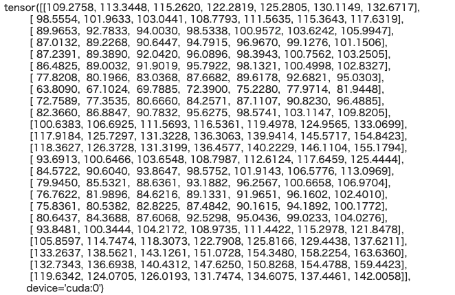
We get predictions of 5 time-series for 24 days.
For each day we get 7 predictions - these are the 7 quantiles:
- [0.02, 0.1, 0.25, 0.5, 0.75, 0.9, 0.98]
We are mostly interested in the 4th quantile which represents, let's say, the 'median loss' fyi, although docs use the term quantiles, the most accurate are percentiles

* Plot

We use the plot_prediction() to create our plots. the plot_prediction() has the extra benefit of adding the attention values.
Note: Our model predicts the next 24 datapoints in one go. This is not a rolling forecasting scenario where a model predicts a single value each time and 'stitiches' all predictions together.

import matplotlib.pyplot as plt

# We create one plot for each consumer( 5 in total).

for idx in range(5): # plot all 5 consumers
  fig, ax = plt.subplots(figsize=(10, 4))
  best_tft.plot_prediction(raw_predictions.x, raw_predictions.output, idx=idx, add_loss_to_title=QuantileLoss(), ax=ax)

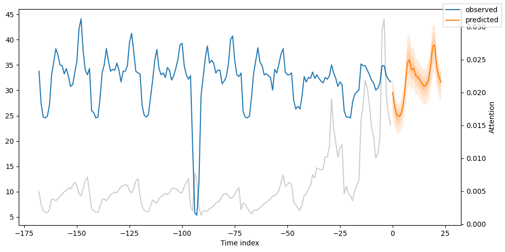
8. Plot Predictions For A Specifit Time Series

Previously, we plot predictions on the validation data using the idx argument, which iterates over all time-series in our dataset. We can be more specific and output predictions on a specifit time-series:

fig, ax = plt.subplots(figsize=(10, 5))

raw_prediction = best_tft.predict(
    training.filter(lambda x: (x.consumer_id == 'MT_004') & (x.time_idx_first_prediction == 26512)),
    mode = 'raw',
    return_x = True
)
best_tft.plot_prediction(raw_prediction.x, raw_prediction.output, idx=0, ax=ax);

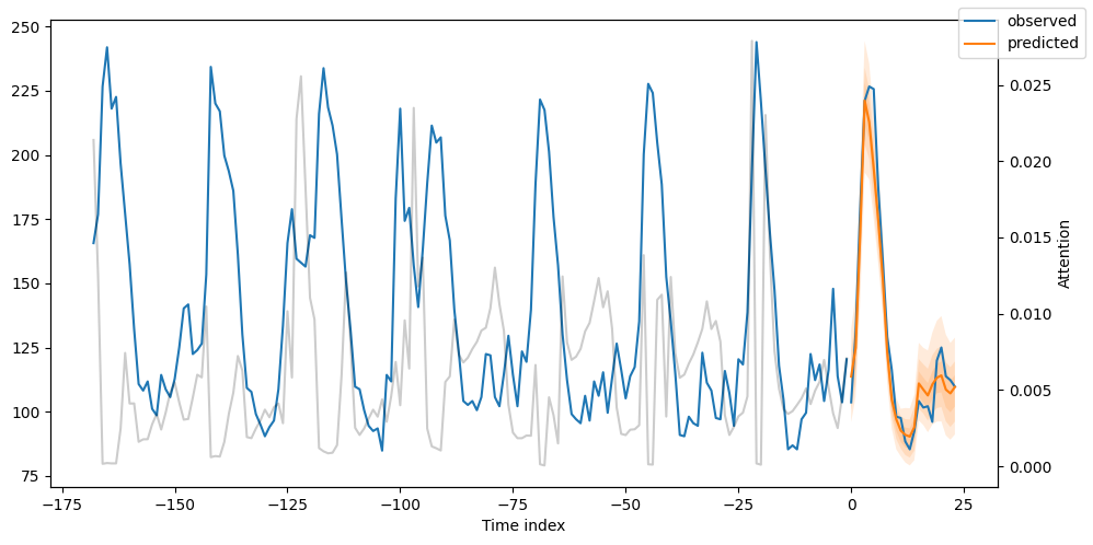
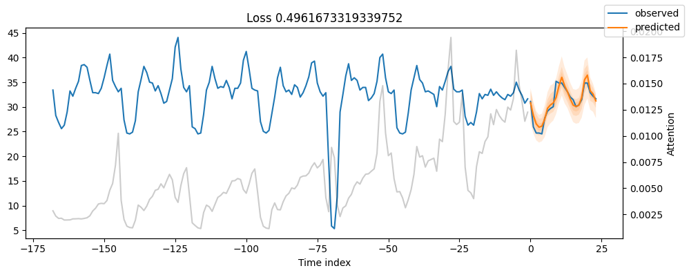
In Upper Figure, we plot the day-ahead of MT_004 consumer for time index=26512.
Remember, our time-indexing column hours_from_start starts from 26304 and we can get predictions from 26388 onwards (because we set earlier min_encoder_length=max_encoder_length // 2 which qeuals 26304 + 168//2 = 26388

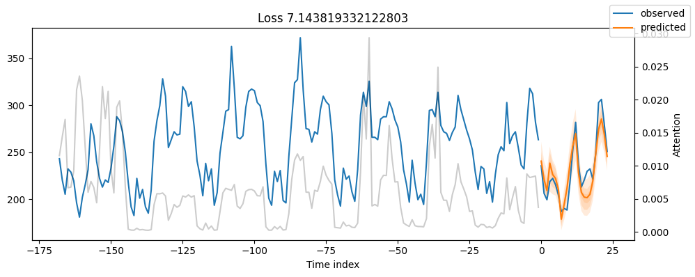
9. Out-of-Sample Forecasts

Let's create out-of-sample predictions, beyond the final datapoint of validation data -which is 2014-09-07 23:00:00
All we have to do is to create a new dataframe that contains:
- The number of N=max_encoder_length past dates, which act as the lookback window - the encoder data in TFT terminology.
- The future dates of size max_prediction_length for which we want to cumpute our predictions - the decoder data.
We can create predictions for all 5 of our time-series, or just one. Following Figure shows the out-of-sample predictions for consumer MT_002.

# encoder data is the last lookback window: we get the last 1 week (168 datapoints) for all 5 consumers = 840 datapoints
encoder_data = time_df[lambda x: x.hours_from_start > x.hours_from_start.max() - max_encoder_length]
last_data = time_df[lambda x: x.hours_from_start == x.hours_from_start.max()]

# decoder_data is the new dataframe for which we will create predictions.
# decoder_data df should be max_prediction_length*consumers = 24*5 = 120 datapoints long : 24 datapoints for each consumer
# we create it by repeating tha last hourly observation of every consumer 24 times since we do not really have new test data
# and later we fix the columns
# df.assign()メソッドは、行や列を追加するメソッド
decoder_data = pd.concat(
    [last_data.assign(date=lambda x: x.date + pd.offsets.Hour(i)) for i in range(1, max_prediction_length + 1)], # date列の作成
    ignore_index = True
)

# fix the new columns( recalc hours_from_start index)
#  tmp['hours_from_start'] = (date - earliest_time).seconds /60/60 + (date - earliest_time).days * 24
decoder_data["hours_from_start"] = (decoder_data['date'] - earliest_time).dt.seconds /60/60 + (decoder_data['date'] - earliest_time).dt.days *24
decoder_data['hours_from_start'] = decoder_data['hours_from_start'].astype('int')
decoder_data['hours_from_start'] += encoder_data['hours_from_start'].max() + 1 - decoder_data['hours_from_start'].min()

decoder_data['month'] = decoder_data['date'].dt.month.astype(np.int64)
decoder_data['hour'] = decoder_data['date'].dt.hour.astype(np.int64)
decoder_data['day'] = decoder_data['date'].dt.day.astype(np.int64)
decoder_data['day_of_week'] = decoder_data['date'].dt.dayofweek.astype(np.int64)

# 予測用のencoderデータを追加
new_prediction_data = pd.concat([encoder_data, decoder_data], ignore_index=True)

new_prediction_data

fig, ax = plt.subplots(figsize=(10, 5))

# create out-of-sample predictions for MT_002
new_prediction_data = new_prediction_data.query("consumer_id == 'MT_002'")
new_raw_predictions = best_tft.predict(new_prediction_data, mode='raw', return_x=True)
best_tft.plot_prediction(new_raw_predictions.x, new_raw_predictions.output, idx=0, show_future_observed=False, ax=ax)

10. Interpretable-Forecasting

Temporal Fusion Transformer provides three types of interpretability
- Seasonality-wise: TFT leverages its novel Interpretable Multi-Head Attention mechanism to calculate the importance of past time steps.
- Feature-wise: TFT leverages its Variable Selection Network module to calculate the importance of every feature.
- Extream events robustness: We can investigate how time series behave during rare events.

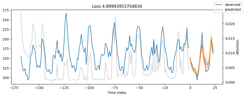
* Seasonality-wise Interpretability

TFT explores the attention weights to understand the temporal patterns across past time step.
On upper graph, the gray lines represent the attention scores. The attention scores reveal how impactful are those time steps when the model outputs its prediction. The small peaks reflect the daily seasonality, while the higher peak towards the end probably implies the weekly seasonality.
TFT has extra advantages:
- We can confirm our model captures the apparent seasonal dynamics of our sequences.
- Our model may also reveal hidden patterns because the attention weights of the current input windows consider all past inputs.
- The attention weights plot is not the same as an autocorrelation plot: The autocorrrelation plot refers to a particular sequence, while the attention weights here focus on the impact of each timestep by looking across all covariates and time series.

* Feature-wise Interpretability

Variable Selection Network component of TFT can easily estimate the feature importance

raw_predictions = best_tft.predict(val_dataloader, mode='raw', return_x=True)
interpretaion = best_tft.interpret_output(raw_predictions.output, reduction='sum')
best_tft.plot_interpretation(interpretaion)

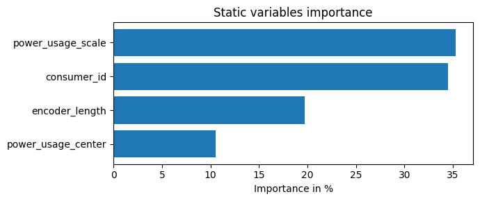
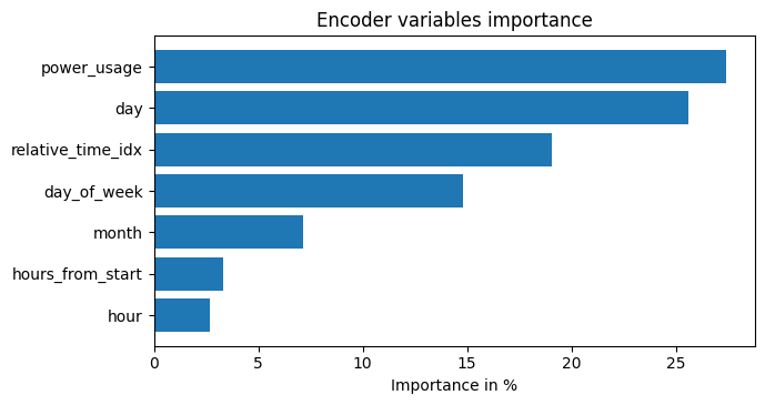
From upper graph, we notice the following:
- The hour, day and day_of_week have strong scores, both as past observations and future covariates. The benchmark in the original paper shares same conclusion.
- The power_usage is obviously the most impactful observed covariate.
- The consumer_id is not very significant here because we use only 5 consumers. In the TFT paper, where the authors use all 370 consumers, this variable is more significant.
Note:If your grouping static variable is not important, it is very likely your dataset can also be modeled equally well by a single distribution model(like ARIMA).

* Extreme Events Detection

Time series are notorious for being susceptible to sudden changes in their properties during rare event.
- notorious: よく知られた、悪名高い、susceptible: 影響を受けやすい、elusive: 捕らにくい
Even worse, those events are very elusive. Imagine if your target varialbe becomes volatile for a breif period because a covariate silently changes behaviour:
- Is this some random noise or a hidden persistent pattern that escapes our model?
- With TFT, we can analyze the robustness of each individual feature across their range of values. Unfortunately, the current dataset does not exhibit volatility or rare events - those are more likely to be found in financial, sales data and so on. we will show how to calculate them

# Analysis on the training set

predictions = best_tft.predict(train_dataloader, return_x=True)
predictions_vs_actuals = best_tft.calculate_prediction_actual_by_variable(predictions.x, predictions.output)
best_tft.plot_prediction_actual_by_variable(predictions_vs_actuals)

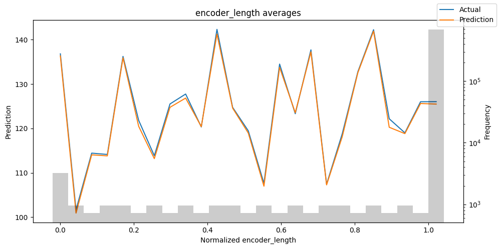
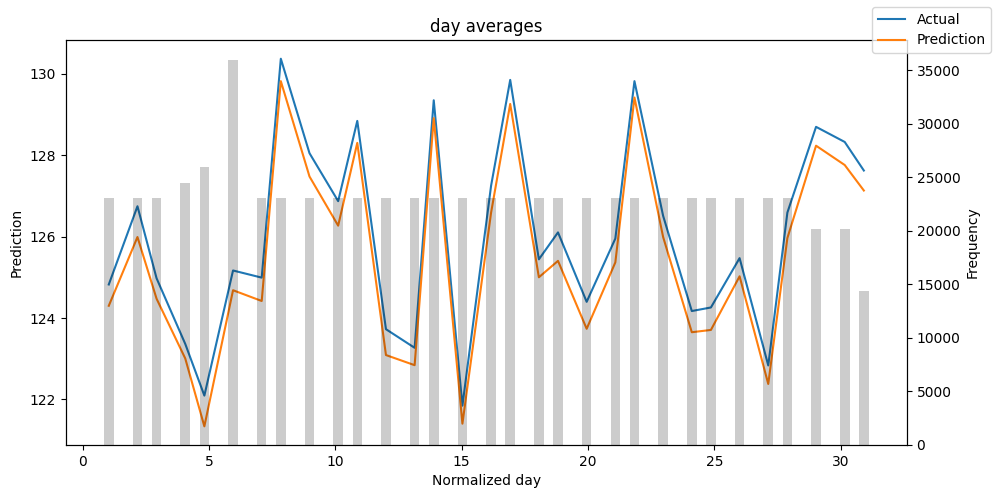
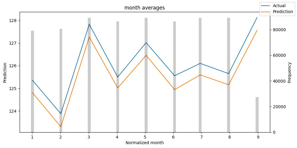
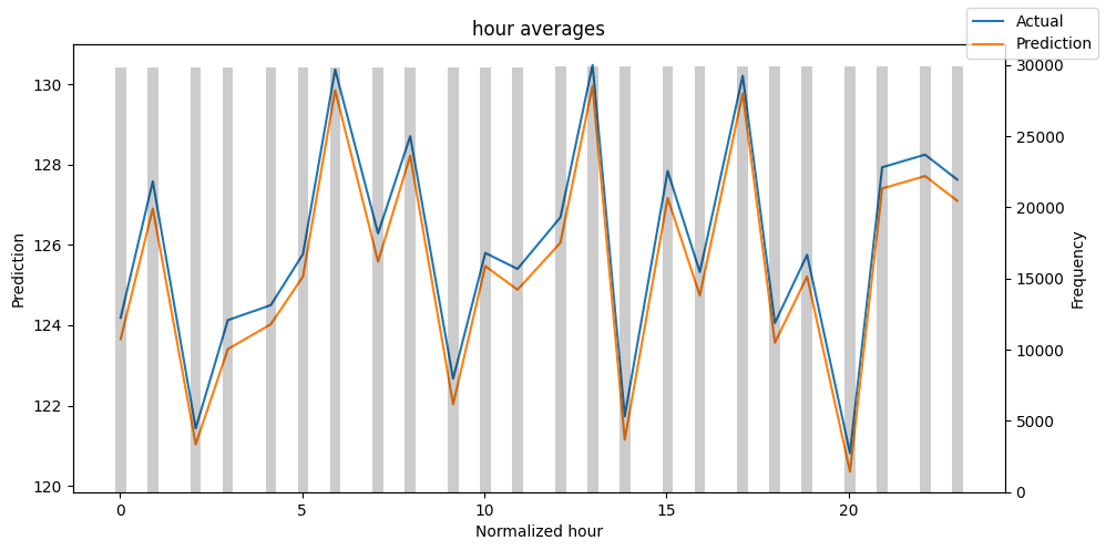
The gray bars denotes the distribution of each variable. One thing I always do is find which values have a low frequency. Then, I check how the model performs in those areas. Hence, you can easily detect if your model captures the behavior of rare events.
In general, you can use this TFT feature to probe your model for weaknesses and proceed to further investigation.

11. Hyperparameter Tuning

We can seamlessly use TFT with Optuna to perform hyperparameter tuning

from pytorch_forecasting.models.temporal_fusion_transformer.tuning import optimize_hyperparameters
import pickle

%%time

# create a new study
study = optimize_hyperparameters(
    train_dataloader,
    val_dataloader,
    model_path='optuna_test',
    n_trials=1,
    max_epochs=1,
    gradient_clip_val_range=(0.01, 1.0),
    hidden_size_range=(30, 128),
    hidden_continuous_size_range=(30, 128),
    attention_head_size_range=(1, 4),
    learning_rate_range=(0.001, 0.1),
    dropout_range=(0.1, 0.3),
    reduce_on_plateau_patience=4,
    use_learning_rate_finder=False
)

# save study results
with open('/content/drive/MyDrive/test_study.pkl', 'wb') as fout:
  pickle.dump(study, fout)

#  print best hyperparameters
print(study.best_trial.params)
'''
# 出力内容
{'gradient_clip_val': 0.27709539558916113, 'hidden_size': 47, 'dropout': 0.17119397185642266, 'hidden_continuous_size': 35, 'attention_head_size': 4, 'learning_rate': 0.019650246121202853}

* TFTの予測値に使われているQuantile Regressionについて

In numerous applications where time series forecasting is involved, the prediction of the target variable is not enough. It is equally important to estimate the uncertainty of the prediction(s). Usually, this comes in the form of prediction intervals. Should we decide to include prediction intervals in the output, linear regression and the mean square error become inapplicable.
Standard linear regression uses the method of ordinary least squares(OLS) to calculate the conditional mean of the target variable across different values of the features. Prediction intervals from the OLS solution are based on the assumption that the residuals have constant variance, which is not always the case.
On the other hand, quantile regression, which is an extension of the standard linear regression, estimates the conditional median of the target variable and can be used when assumptions of linear regression are not met.
Apart from the median, quantile regression can also calculate the 0.25 and 0.75 quantiles (or any precentile for that matter) which means the model has the ability to output a prediction interval around the actual prediction.
Following graph shows an example of how quantiles/percentiles look like in a regression problem.
Given y and ^y the actual value and the prediction respectively, and q a value for the quantile between 0 and 1, the quantile loss function is define as:
- QL(y, ^y, q) = max[q(y - ^y), (1 - q)(y - ^y)]
As the value of q increase, overestimations are penalized by a larger factor compared to underestimations. For instance, for q equal to 0.75, overstimations will be penalized by a factor of 0.75, and underestimations by a factor of 0.25. That's how the prediction intervals are created.
The temporal Fusion Transformer implementation is tarined by minimizing the quantile loss summed across q ∈ [0.1, 0.5, 0.9]. This is done for benchmarking purposes, in order to match the experimental configuration used by other poplular models. Also, it goes without saying that the use of quantile loss is not exclusive - other types of loss functions can be used such as MSE, MAPE and so on.

* encoder-decoderモデルで、学習データ、バリデーションデータ(early stopping用)、テストデータを用意する時の注意点(TFTコード例での、train_cutoffについて)

以下は、テキストより抜粋（テキストでは、ウインドウサイズ96ステップで1ステップを予測するTFTモデルを作成)
- We have chosen to have 2 days(96 timesteps) as the window and predict one single step ahed. And to enable early stopping, we should need a validation set as well. Early stopping is a way of regularization where we keep monitoring the validation loss and stop tarining when the validation loss starts to increase.
- We have selected the last day of taining(48 timesteps) as the validation data and 1 whole month as the final data.
- But when we these dataframes, we need to take care of something: we have chosen 2 days as our history, and to forecast the first timestep in the validation or test set, we need the last 2 days of history along with it. So we split our dataframes as shown in the following diagram:
予測時に、2日分のエンコーダ用データが必要なので、val, testそれぞれに予測期間前2日分のデータを付与している。

You get articles that match your needs
You can efficiently read back useful information
You can use dark theme

What you can do with signing up