Objective

To explore Individual Conditional Expectation (ICE) and run it in R script. This article is based on information in 「機械学習を解釈する技術 ~Techniques for Interpreting Machine Learning~」by Mitsunosuke Morishita. In this book, the author does not go through all the methods by R, so I decided to make a brief note with an R script.

SHapley Additive exPlanations (SHAP) is a method to understand how our AI model came to a certain decision. For example, if your task is to make AI for the loan screening process, you need to make sure why your AI came up to the conclusion because your applicant would desperate to know why they failed. The idea of SHAP is to allocate/calculate credits for each explanatory variable on the prediction. For example, in cooperative game theory, a player is able to choose "join" or "not join" the game. And if all players are "join" the game except player A, the difference between the result of the game within all players and the game without player A is going to be credited to player A. SHAP does a similer process to the model to help us to understand the behavior of the model.

Additive Feature Attribution Method

SHAP computes credits by calculating the difference of the overall prediction and an individual prediction. For example, a model $\hat{f}(X)$ with explanatory variable $X = (X_1,...,X_J)$. So explanatory variables for observation $i$ are $x_i=(x_{i,1}...,x_{i,J})$. In SHAP, the credits are break down into the addition form.

$$
\hat{f}(x_i) - \mathbb{E}\big[\hat{f}(X)\big] = \sum_{j = 1}^{J} \phi_{i,j}
$$

Breaking down into summation from called Additive Feature Attribution Method and SHAP is one of the Additive Feature Attribution Methods. Often, by setting $\phi_0 = \mathbb{E}\big[\hat{f}(X)\big]$ SHAP is notated as

$$
\hat{f}(x_i) = \phi_{0} - \sum_{j = 1}^{J} \phi_{i,j}
$$

For example, let's say our goal is to predict annual salary from education, job title, job position, and English skill. The prediction formula would be

$$
\hat{f}(x_i) = \phi_0 + \phi_i, education + \phi_i title + \phi_i position + \phi_i english
$$

In this particular observation, we get someone who got a Master's degree, works as Data Scientist, is a Manager, and does not speak English. And the predicted salary is 10 million yen.

According to our AI model, if he practices his English, he has more chance to be predicted a higher salary.

Shapley Value

The Shapley value is a solution concept used in game theory that involves fairly distributing both gains and costs to several actors working in a coalition. Game theory is when two or more players or factors are involved in a strategy to achieve a desired outcome or payoff. -Will Kenton(investopedia).

Let's say there are three players A, B, and C in some cooperative game, and we want to somehow calculate the contributions of each player. Here is a table of final scores with a list of players in the game.

Player	Score
A	6
B	4
C	2
A,B	20
A,C	15
B,C	10
A,B,C	24

To calculate the contribution, we use marginal contribution. Marginal contribution calculates one's effort by getting the average of the difference between the game scores with and without a certain player. For example, if you want to calculate marginal contribution for player A,

Game 1
Player A plays the game aloe, A gets a score of 6.
None -> A
$Contribution_A = 6 - 0 = 6$

Game 2
Player B plays the game aloe(4), but A gets into the game. A and B gets score of 20.
B -> A,B
$Contribution_A = 20 - 4 = 16$

Game 3
Player C plays the game aloe(2), but A gets into the game. A and C gets score of 15.
C -> A,C
$Contribution_A = 15 - 2 = 13$

Game 4
Player B and C plays the game (10), A gets into the game. A,B, and C gets score of 24.
B,C -> A,B,C
$Contribution_A = 24 - 10 = 14$

Pay attention to the fact that the contribution of A changes who's in the game already. Therefore, we need to average each contribution.

Here is a table of marginal contributions with all possible participation orders.

Participation Order	Contribution A	Contribution B	Contribution C
A-B-C	6	14	4
A-C-B	6	9	9
B-A-C	16	4	4
B-C-A	14	4	6
C-A-B	13	9	2
C-B-A	14	8	2

By taking the average we can calculate the Shapley Value

$$
\phi_{A} = \dfrac{6+6+16+14+13+14}{6}=11.5
$$

Formula for Shapley Value

$$
\phi_{j} = \dfrac{1}{|\mathbf{J}|!} \sum_{\mathbf{S}\subseteq\mathbf{J}-j} (|\mathbf{S}|!(|\mathbf{J}|-|\mathbf{S}|-1)!) (v(\mathbf{S}\cup{j})-v(\mathbf{S}))
$$

$\mathbf{J} = \{1,...,J\}$ is a set of players.

In the case above, $\mathbf{J} = \{A,B,C\}$

$|\mathbf{J}|$ is the number of components in the set $\mathbf{J}$.

In the case above, $|\mathbf{J}| =3$

$\mathbf{S}$ is a set of sets that deducts player $j$ from $\mathbf{J}$.

Thinking about shapely value of A, $\mathbf{S}$ is $\emptyset,\{B\},\{C\},\{B,C\}$

$|\mathbf{S}|$ is number of components in the set $\mathbf{S}$.

In the case $\emptyset,\{B\},\{C\},\{B,C\}$, $|\mathbf{S}|$ would be $0,1,1,2$

$v$ is a game score.

If A and B are in the game, the score would be notated as $v(\{A,B\})$

$v(\mathbf{S}\cup\{j\}) - v(\mathbf{S})$ is difference of the scores when player $j$ is in and out of the game.

Execution with Real Data

Now, let's see how to run PFI with actual dataset.

Get Dataset

# Set up
library(mlbench)
library(tidymodels)
library(DALEX)
library(ranger)
library(Rcpp)
library(corrplot)
library(ggplot2)
library(gridExtra)
library(SHAPforxgboost)

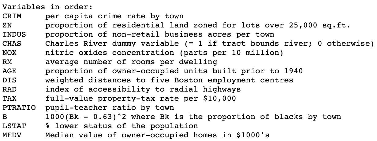
data("BostonHousing")
df = BostonHousing

Overview of the Dataset

Here is an overview of the dataset

Build a Model

We won't cover building a model in this article. I used the XGBoost model.

split = initial_split(df, 0.8)
train = training(split)
test = testing(split)

model = rand_forest(trees = 100, min_n = 1, mtry = 13) %>% 
  set_engine(engine = "ranger", seed(25)) %>% 
  set_mode("regression")

fit = model %>% 
  fit(medv ~., data=train)
fit

Predict medv

result = test %>% 
  select(medv) %>% 
  bind_cols(predict(fit, test))

metrics = metric_set(rmse, rsq)

result %>% 
  metrics(medv, .pred)

Interpret SHAP

Use the function explain to create an explainer object that helps us to interpret the model.

explainer = fit %>% 
  explain(
    data = test %>% select(-medv),
    y = test$medv
  )

Use predict_parts function to get SHAP plot.

new_observation: Set an observation which you want to calculate SHAP
type: Set the method
B: Number of trials of picking ways of "Participation Order"

shap = explainer %>% 
  predict_parts(
    new_observation = test %>% dplyr::slice(11),
    type = "shap",
    B = 25)
plot(shap)

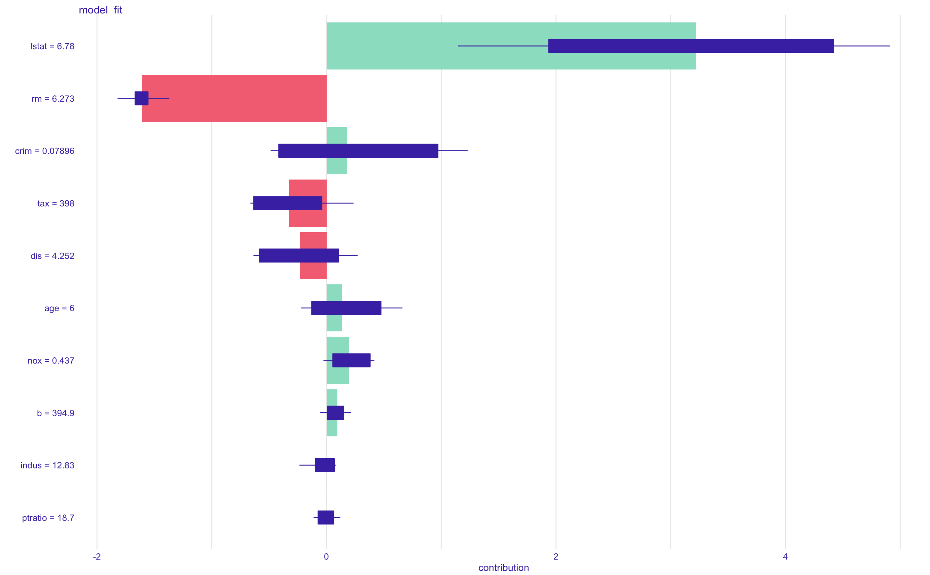
By looking at the plot, we can tell that lstat has the highest contribution to the prediction. To interpret, lstat contributes medv to be high, but rm contributes medv to be low, and so on...

FYI

Method	Function
Permutation Feature Importance(PFI)	model_parts()
Partial Dependence(PD)	model_profile()
Individual Conditional Expectation(ICE)	predict_profile()
SHAP	predict_parts()

Global Feature Importance

The SHAP approach can be used to get a macro/overview of the model by taking an absolute average of the SHAP value for all observations. Thank you to Yang Liu for making this all-in-one package that manages to build a model and plot SHAP plot. For more information, visit here

library(tidyverse)
library(xgboost)
library(caret)

dummy <- dummyVars(" ~ .", data=df)
newdata <- data.frame(predict(dummy, newdata = df)) %>% 
  select(-medv)

model_wine <- xgboost(data = as.matrix(newdata), 
                      label = df$medv, 
                      objective = "reg:squarederror", 
                      nrounds = 100)

shap_result_wine <- shap.score.rank(xgb_model = model_wine, 
                                    X_train = as.matrix(newdata),
                                    shap_approx = F
                                    )

var_importance(shap_result_wine, top_n = ncol(d_mx) - 1 )

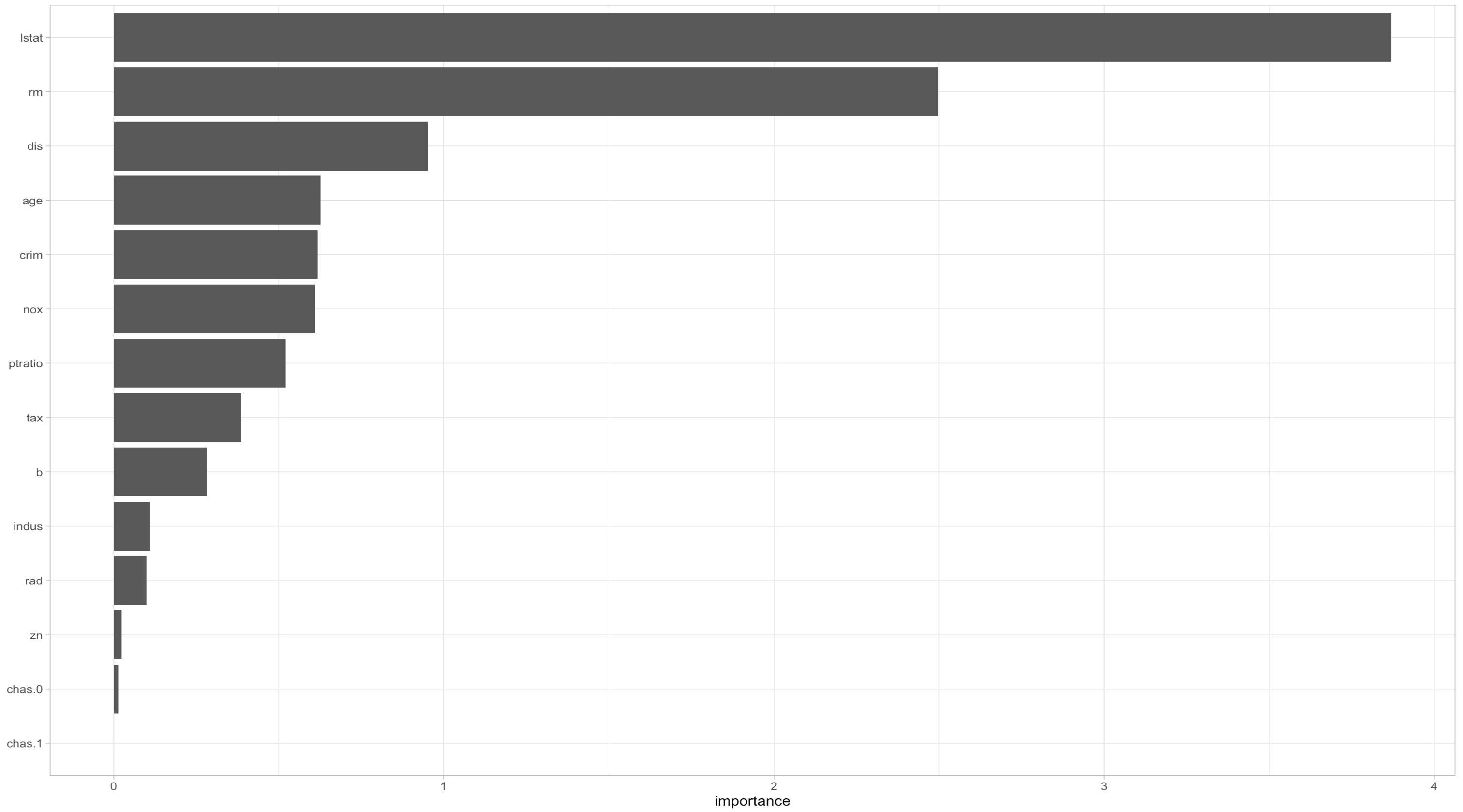
Just like that one observation, lstat and rm are the most important feature in the whole dataset.

Conclution

SHAP is a sufficient method to observe the variable importance of each observation. At the same time, SHAP also can be helpful to get an overview of the whole model. However, SHAP cannot explain the relationship between explanatory variable and response variable, which can be explain with ICE.

【R/English】SHapley Additive exPlanations (SHAP)