この記事ではグラフ解析ライブラリgraph-toolで行う典型的な処理をまとめた。
特にグラフの構築と、次数分布などのグラフの基本的な統計量を計算する方法をまとめる。

動作確認環境は以下の通り

python 3.9.0
graph-tool 2.35
numpy, matplotlib

以後のサンプルコードでは、前提条件として以下のモジュールをimportしている。

import graph_tool.all as gt
import numpy as np
import matplotlib.pyplot as plt

基本操作

グラフの構築

グラフオブジェクトの作成

g = gt.Graph()
# => <Graph object, directed, with 0 vertices and 0 edges, at 0x7fbf8897c100>

デフォルトで有向グラフになる。undirected graphを構築するにはdirected=Falseを引数で指定する

ug = gt.Graph(directed=False)

ノード追加

v = g.add_vertex()         # => <Vertex object with index '0' at 0x7fbfd8c718d0>
vlist = g.add_vertex(3)   # 複数のノードの追加
# => [<Vertex object with index '1' at 0x7fbfd8c71690>,  <Vertex object with index '2' at 0x7fbfd8c71b10>,   <Vertex object with index '3' at 0x7fbfd8c71bd0>]

# get the number of vertices
g.num_vertices()   # => 4

# get vertex object by index
v2 = g.vertex(2)   # => <Vertex object with index '2' at 0x7fbfd8c71b10>

この例でみたようにNodeをindexから取得するときには g.vertex(idx) とすれば取得することができる。
逆にvertex v があるときにそこからindexを取得する際には int(v) と整数に変換すれば取得できる。

エッジ追加

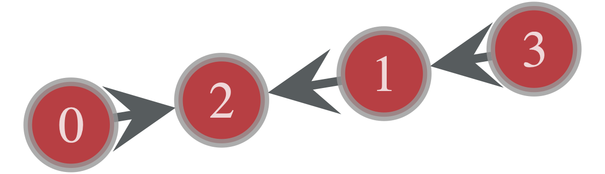
e = g.add_edge(g.vertex(0), g.vertex(2))                 # => 0,2 の間にエッジを作る
( e.source(), e.target() )                # => vertex0, vertex2 をそれぞれ取得

# 短縮してintegerを引数に渡すこともできる
e1 = g.add_edge(3, 1)
e2 = g.add_edge(1, 2)

試しにこの状態で可視化してみると以下のようになる。

gt.graph_draw(g, vertex_text = g.vertex_index)

同じノードペアに対して複数のエッジ(multiedge)を作成したり、始点と終点が同一な self-loopを作ることも同様の手順でできる。

イテレーション

エッジおよびノードに対してイテレーションする処理は以下のように書ける

# iterations over vertices
for v in g.vertices():
    for e in v.out_edges():
        print(e.source(), e.target())

# iterations over edges
for e in g.edges():
    print(e.source(), e.target())

エッジ数、ノード数の取得

g.num_vertices()   # => 4
g.num_edges()     # => 3

属性の追加

reference : https://graph-tool.skewed.de/static/doc/quickstart.html#property-maps

ノードおよびエッジに属性を指定することができ、それぞれVertexProperty, EdgePropertyと呼ばれる。（グラフ全体に対しても属性 GraphProperty を付与することができるが、主に使うのはVertexとEdgeだけだろう）

例えば、重み付きのグラフのエッジの重みはdouble型のEdgePropertyとして指定することができる。
int, doubleといった数値的な型だけではなく、bool, string, vector<int>, vector<double>, object といった様々な型の属性を付与することができる。
たとえばノードの名前をstring型のVertexPropertyとして保持したり、マルチレイヤーネットワークのリンクのレイヤーの情報をint型のEdgePropertyとして持つことができる。

たとえば重み付きグラフを構築する手順は以下の通りになる。

g = gt.Graph()
g.ep["weight"] = g.new_edge_property("double")                            # `ep` (edge property)の"weight" という名前でdouble型のedge propertyを作成
g.list_properties()
#  =>     weight         (edge)    (type: double)

以後、g.ep.weight でアクセスでき、さらにg.ep.weight.a で内部のnumpy.arrayが取得できる

g.ep.weight                      # => <EdgePropertyMap object with value type 'double', for Graph 0x7fbf8897c100, at 0x7fbfcb2e3ee0>
g.ep.weight.a                 # PropertyArray([0., 0., 0.])

要素にアクセスするには[] に edge (vertex) を渡す。
EdgePropertyおよびVertexPropertyはedge(vertex)を引数にして要素アクセスできる配列のようなものだと考えておけば良い。

e1 = g.edge( g.vertex(0), g.vertex(2) )    # node-(0,2) の間のedgeを取得
g.ep.weight[e]          # => weight of edge e

基本統計量の計算

以後、以下のサンプルデータを用いて説明する。このサンプルデータにはg.ep.value に重みが格納されている。

g = gt.collection.data["celegansneural"]

degree distribution

vertex_hist メソッドで取得する。in-degree, out-degree, total-degreeの場合、第２引数に"in", "out", "total" という文字列をそれぞれ渡す。
参考 : https://graph-tool.skewed.de/static/doc/stats.html#graph_tool.stats.vertex_hist

pk,k = gt.vertex_hist(g, "out")

plt.xlabel("degree")
plt.ylabel("frequency")
plt.plot(k[:-1], pk)               # `k`の最後の１要素は除く

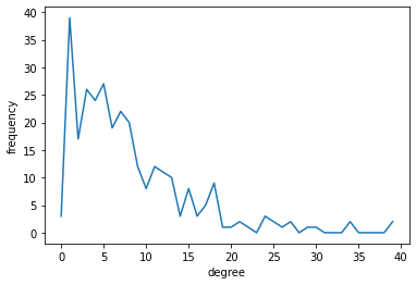
pk, k ともにnumpy.arrayで返るが、pkの方がサイズが一つ大きい。
これはkの方に、それぞれのbinの最大値、最小値が入るため。プロットするときにはkの最後の要素を取り除く必要がある。

第二引数に文字列ではなくVertexPropertyを渡すことで、次数以外の任意のVertexPropertyの分布を計算することもできる。

average_degree

avg,sdv = gt.vertex_average(g, "out")          # => (7.942760942760943, 0.39915717608995005)

第二引数に "in", "out", "total" の文字列を指定すると、それぞれin-degree, out-degree, total-degree の平均値が計算され、平均と標準偏差が返り値として得られる。

また、次数以外にもVertexのPropertyの平均値も同様に計算することができる。

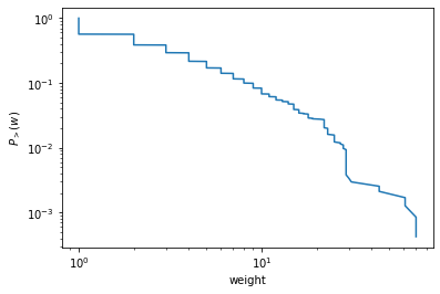
edge weight distribution

参考: https://graph-tool.skewed.de/static/doc/stats.html#graph_tool.stats.edge_hist

pw,w = gt.edge_hist(g, g.ep.value)
# =>
(array([0.000e+00, 1.023e+03, 4.250e+02, 2.200e+02, 1.820e+02, 1.070e+02,
        7.000e+01, 6.000e+01, 3.800e+01, 3.800e+01, 3.700e+01, 1.500e+01,
        1.600e+01, 7.000e+00, 1.000e+01, 2.000e+01, 1.100e+01, 2.000e+00,
        1.100e+01, 2.000e+00, 0.000e+00, 1.000e+00, 1.700e+01, 1.000e+01,
        0.000e+00, 9.000e+00, 0.000e+00, 2.000e+00, 4.000e+00, 1.400e+01,
        1.000e+00, 1.000e+00, 0.000e+00, 0.000e+00, 0.000e+00, 0.000e+00,
        0.000e+00, 0.000e+00, 0.000e+00, 0.000e+00, 0.000e+00, 0.000e+00,
        0.000e+00, 0.000e+00, 2.000e+00, 0.000e+00, 0.000e+00, 0.000e+00,
        0.000e+00, 0.000e+00, 0.000e+00, 0.000e+00, 0.000e+00, 0.000e+00,
        0.000e+00, 0.000e+00, 0.000e+00, 0.000e+00, 0.000e+00, 0.000e+00,
        0.000e+00, 2.000e+00, 0.000e+00, 0.000e+00, 0.000e+00, 0.000e+00,
        0.000e+00, 0.000e+00, 0.000e+00, 0.000e+00, 2.000e+00]),
 array([ 0.,  1.,  2.,  3.,  4.,  5.,  6.,  7.,  8.,  9., 10., 11., 12.,
        13., 14., 15., 16., 17., 18., 19., 20., 21., 22., 23., 24., 25.,
        26., 27., 28., 29., 30., 31., 32., 33., 34., 35., 36., 37., 38.,
        39., 40., 41., 42., 43., 44., 45., 46., 47., 48., 49., 50., 51.,
        52., 53., 54., 55., 56., 57., 58., 59., 60., 61., 62., 63., 64.,
        65., 66., 67., 68., 69., 70., 71.]))

vertex_histのedgeバージョン。任意のEdgePropertyの分布を計算することができる。

また、complementary cumulative distribution function は以下のようにプロットできる

# complementary cumulative distribution function
weights = np.sort(g.ep.value.a)
ccdf = np.linspace(1.0, 0.0, num=g.num_edges(), endpoint=False)
plt.xlabel("weight")
plt.ylabel(r"$P_{>}(w)$")
plt.xscale("log")
plt.yscale("log")
plt.plot(weights, ccdf)

average edge weight

vertex_averageのedgeバージョン。

gt.edge_average(g, g.ep.value)

参考 : https://graph-tool.skewed.de/static/doc/stats.html#graph_tool.stats.edge_average

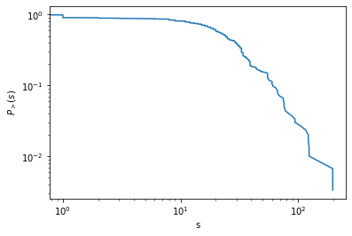
node strength

node strengthは自分でイテレートして計算する必要がある。
"double"のvertex_propertyを作成して、その中にnode strengthを格納する。

out_strength = g.new_vertex_property("double")
for v in g.vertices():
    weights = [g.ep.value[e] for e in v.out_edges()]
    out_strength[v] = np.sum(weights)

ps,s = gt.vertex_hist(g, out_strength)

# plot of complementary cumulative distribution function
s = np.sort(out_strength.a)
ccdf = np.linspace(1.0, 0.0, num=g.num_vertices(), endpoint=False)
plt.xlabel("s")
plt.ylabel(r"$P_{>}(s)$")
plt.xscale("log")
plt.yscale("log")
plt.plot(s, ccdf)

clustering coefficient

参考 : https://graph-tool.skewed.de/static/doc/clustering.html#graph_tool.clustering.global_clustering

gt.global_clustering(g)              # => (0.19795997218143885, 0.027169317947021772)

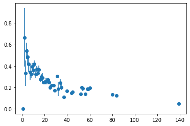
clustering spectrum c(k)

nodeにおける属性間の相関をみるにはavg_combined_corrを使う。
degreeとlocal clustering coefficientだけでなく、任意のVertexProperty間の相関を計算できる。
参考 : https://graph-tool.skewed.de/static/doc/correlations.html#graph_tool.correlations.avg_combined_corr

# correlation between k and local clusteirng
gt.local_clustering(g)                 # => double type の VertexProperty

h = gt.avg_combined_corr(g, "total", gt.local_clustering(g))
plt.errorbar( h[2][:-1], h[0], yerr=h[1], fmt="o")

h は (bin, average, stddev) のタプル

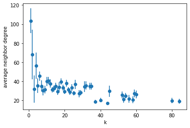
degree correlation

参考 : https://graph-tool.skewed.de/static/doc/correlations.html#graph_tool.correlations.avg_neighbor_corr

隣接ノード間のVertexPropertyの相関を計算することができる。文字列"in", "out", "total" を引数に渡すと次数相関を計算できる。

# average degree correlation
knn = gt.avg_neighbor_corr(g, "total", "total")
plt.xlabel("k")
plt.ylabel("average neighbor degree")
plt.errorbar( knn[2][:-1], knn[0], yerr=knn[1], fmt="o")

centrality

参考 : https://graph-tool.skewed.de/static/doc/centrality.html

さまざまなcentralityの指標を計算できるが、ここではpagerankを計算してみよう。
gt.pagerankでpagerankを計算してVertexPropertyとして取得できる。その値に応じて色をつけて描画してみる。

prc = gt.pagerank(g, weight = g.ep.value)
gt.graph_draw(g, vertex_fill_color = prc, pos = g.vp.pos)

pagerankの他にもbetweeness centrality, Katz centrality, eigen-vector centrality など一通り揃っている。

graph-toolチートシート（グラフ構築、統計量編）