能動的推論エージェントのモニタリング機能の実装を検討します。
モニタリング指標
このモニタリングシステムの観測指標は以下の通りとします。
| 指標名 | 意味する内容 |
|---|---|
|
Belief States Evolution 信念状態の推移 |
・ エージェントの状態認識の推移 ・ 1に近いほどその状態である確信が強い ・ 0に近いほどその状態でないと判断 |
|
Belief Stability 信念の安定性の時系列変化 |
・ 値が小さいほど信念が安定 ・ 値が大きいほど信念が不安定 ・ 学習の収束度を示す指標 |
|
Action Selection Probability 行動選択確率 |
・ 行動選択の偏りを表示 ・ 均等な分布は探索的な行動を示す ・ 偏りは特定行動への収束を示す |
|
Action Selection Trend 行動選択の傾向変化 |
・ 行動選択戦略の変化を示す ・ 高い値は特定行動の優位性 ・ 変動は戦略の探索を示す |
|
Free Energy Evolution 変分自由エネルギーの推移 |
・ モデルの予測精度を示す ・ 値が小さいほど予測が正確 ・ 上昇は予測精度の低下を示す |
|
Prediction Error 予測誤差 |
・ 予測の正確さを直接的に示す ・ 値が小さいほど予測が正確 ・ 変動は予測の不安定さを示す |
実装
import numpy as np
import matplotlib.pyplot as plt
import seaborn as sns
from collections import defaultdict

class MonitoringSystem:
    def __init__(self):
        """モニタリングシステムの初期化"""
        self.history = defaultdict(list)

    def record(self, **kwargs):
        """
        データの記録

        Parameters:
        -----------
        **kwargs : 記録するデータの名前と値のペア
        """
        for key, value in kwargs.items():
            self.history[key].append(value)

    def analyze_beliefs(self):
        """信念状態の分析"""
        beliefs = np.array(self.history['beliefs'])

        # 基本統計量の計算
        mean_beliefs = np.mean(beliefs, axis=0)
        std_beliefs = np.std(beliefs, axis=0)

        # 信念の安定性(分散の時間変化)
        stability = np.array([np.var(beliefs[max(0, i-10):i+1], axis=0)
                            for i in range(len(beliefs))])

        return {
            'mean_beliefs': mean_beliefs,
            'std_beliefs': std_beliefs,
            'stability': stability
        }

    def analyze_actions(self):
        """行動選択の分析"""
        actions = np.array(self.history['actions'])

        # 行動の頻度分析
        action_counts = np.bincount(actions)
        action_probs = action_counts / len(actions)

        # 行動の時間的変化(移動平均)
        window_size = 10
        action_trends = np.array([np.mean(actions[max(0, i-window_size):i+1])
                                for i in range(len(actions))])

        return {
            'action_probs': action_probs,
            'action_trends': action_trends
        }

    def analyze_learning(self):
        """学習過程の分析"""
        free_energy = np.array(self.history['free_energy'])
        observations = np.array(self.history['observations'])

        # 自由エネルギーの変化
        fe_trend = np.array([np.mean(free_energy[max(0, i-10):i+1])
                            for i in range(len(free_energy))])

        # 予測誤差の計算
        predicted_obs = np.array(self.history['predicted_observations'])
        prediction_errors = np.abs(predicted_obs - observations)

        return {
            'fe_trend': fe_trend,
            'prediction_errors': prediction_errors
        }

    def plot_comprehensive_analysis(self):
        """包括的な分析結果の可視化"""
        belief_analysis = self.analyze_beliefs()
        action_analysis = self.analyze_actions()
        learning_analysis = self.analyze_learning()

        fig = plt.figure(figsize=(15, 12))
        gs = fig.add_gridspec(3, 2)

        # 信念状態の推移
        ax1 = fig.add_subplot(gs[0, 0])
        beliefs = np.array(self.history['beliefs'])
        for i in range(beliefs.shape[1]):
            ax1.plot(beliefs[:, i], label=f'State {i}')
        ax1.set_title('Belief States Evolution')
        ax1.set_xlabel('Time Step')
        ax1.set_ylabel('Probability')
        ax1.legend()

        # 信念の安定性
        ax2 = fig.add_subplot(gs[0, 1])
        for i in range(belief_analysis['stability'].shape[1]):
            ax2.plot(belief_analysis['stability'][:, i],
                    label=f'State {i} Stability')
        ax2.set_title('Belief Stability')
        ax2.set_xlabel('Time Step')
        ax2.set_ylabel('Variance')
        ax2.legend()

        # 行動選択の傾向
        ax3 = fig.add_subplot(gs[1, 0])
        ax3.bar(range(len(action_analysis['action_probs'])),
                action_analysis['action_probs'])
        ax3.set_title('Action Selection Probability')
        ax3.set_xlabel('Action')
        ax3.set_ylabel('Probability')

        # 行動の時間的変化
        ax4 = fig.add_subplot(gs[1, 1])
        ax4.plot(action_analysis['action_trends'])
        ax4.set_title('Action Selection Trend')
        ax4.set_xlabel('Time Step')
        ax4.set_ylabel('Action Probability')

        # 自由エネルギーの推移
        ax5 = fig.add_subplot(gs[2, 0])
        ax5.plot(learning_analysis['fe_trend'])
        ax5.set_title('Free Energy Evolution')
        ax5.set_xlabel('Time Step')
        ax5.set_ylabel('Free Energy')

        # 予測誤差の推移
        ax6 = fig.add_subplot(gs[2, 1])
        ax6.plot(learning_analysis['prediction_errors'])
        ax6.set_title('Prediction Error')
        ax6.set_xlabel('Time Step')
        ax6.set_ylabel('Error')

        plt.tight_layout()
        plt.show()

    def save_analysis_report(self, filename='analysis_report.txt'):
        """分析レポートの保存"""
        belief_analysis = self.analyze_beliefs()
        action_analysis = self.analyze_actions()
        learning_analysis = self.analyze_learning()

        with open(filename, 'w') as f:
            f.write("Active Inference Agent Analysis Report\n")
            f.write("=====================================\n\n")

            f.write("1. Belief State Analysis\n")
            f.write("-----------------------\n")
            f.write(f"Mean beliefs: {belief_analysis['mean_beliefs']}\n")
            f.write(f"Belief stability: {np.mean(belief_analysis['stability'])}\n\n")

            f.write("2. Action Selection Analysis\n")
            f.write("---------------------------\n")
            f.write(f"Action probabilities: {action_analysis['action_probs']}\n")
            f.write(f"Action trend stability: {np.std(action_analysis['action_trends'])}\n\n")

            f.write("3. Learning Process Analysis\n")
            f.write("---------------------------\n")
            f.write(f"Mean free energy: {np.mean(learning_analysis['fe_trend'])}\n")
            f.write(f"Mean prediction error: {np.mean(learning_analysis['prediction_errors'])}\n")
使用例
# 使用例
def demo_monitoring():
    # モニタリングシステムの初期化
    monitor = MonitoringSystem()

    # シミュレーションデータの生成(例)
    n_steps = 100
    n_states = 3

    # ダミーデータの生成と記録
    for t in range(n_steps):
        beliefs = np.random.dirichlet(np.ones(n_states))
        action = np.random.choice([0, 1])
        free_energy = np.random.normal(-1, 0.1)
        observation = np.random.randint(0, 4)
        predicted_obs = np.random.randint(0, 4)

        monitor.record(
            beliefs=beliefs,
            actions=action,
            free_energy=free_energy,
            observations=observation,
            predicted_observations=predicted_obs
        )

    # 分析の実行と可視化
    monitor.plot_comprehensive_analysis()
    monitor.save_analysis_report()

if __name__ == "__main__":
    demo_monitoring()
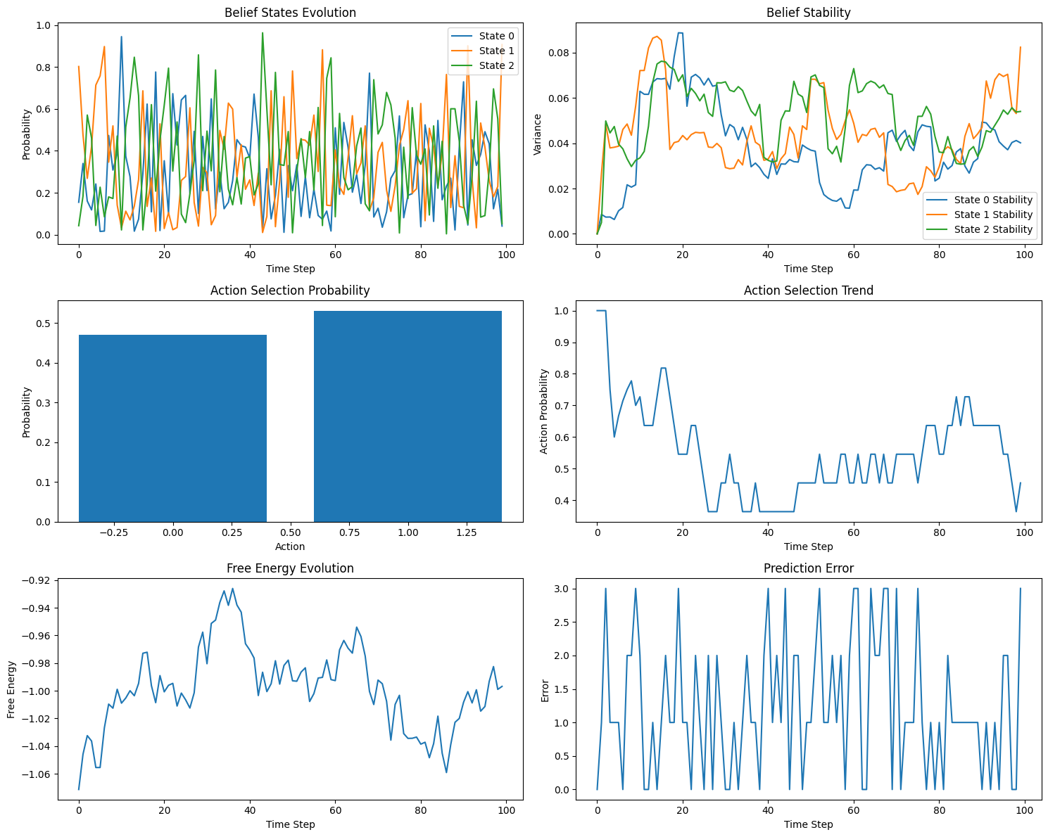
各グラフセットが6つの指標を示しています。
このグラフセットから以下の特徴が読み取れます:
- 行動選択は比較的バランスが取れている
- エージェントの学習は完全な収束には至っていない
- 信念状態は継続的に更新され、固定化されていない
- 予測精度に改善の余地がある