文系エンジニア、ランダムウォークを学ぶ

ランダム・ウォーク理論とは

ランダム・ウォーク理論は、時間の経過と共に発生するランダムな変化をモデル化した理論です。
ランダム・ウォーク理論の主要な要素には以下のものがあります：

• 独立したステップ: 各ステップは前のステップから独立しています
• ランダムな方向性: 移動する方向は完全にランダムです
• ランダムな距離: 移動する距離もランダムに決まります

ランダム・ウォーク理論の登場の背景

ランダム・ウォーク理論の登場背景には、科学と数学の複数の分野が関係しています。この理論は、自然現象のランダム性を理解し、モデル化するために発展しました。

物理学における背景

1827年、植物学者のロバート・ブラウンが花粉粒子が水中でランダムに動く現象（ブラウン運動）を発見。これがランダム・ウォーク理論の初期の基盤を形成しました。
その後19世紀後半、物理学者たちは分子のランダムな運動がマクロスケールでの現象にどのように影響するかを理解し始めました。

数学と確率論の進展

20世紀初頭、確率論が数学の一分野として確立されました。ランダム・ウォークは確率論の基本的なモデルとなり、数学者たちによって形式化されました。
ロシアの数学者アンドレイ・マルコフは、ランダム・ウォークがマルコフ連鎖の特別なケースであることを示しました。

プロットしてみよう

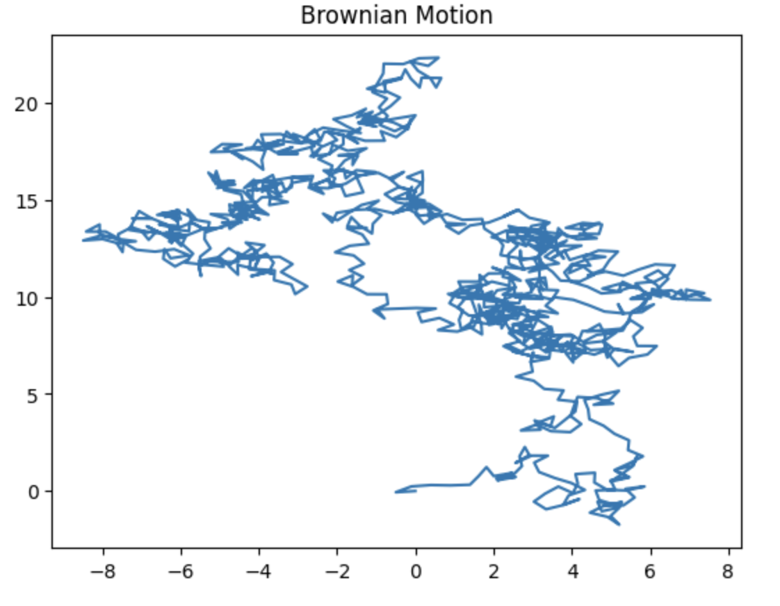
ブラウン運動（ブラウン粒子の動きを模倣したランダムウォーク）のシミュレーションを行い、それをプロットします。

import numpy as np
import matplotlib.pyplot as plt

# ブラウン運動のパラメータ
n_steps = 1000
step_size = 0.5

# 初期位置
x, y = 0, 0
x_positions, y_positions = [x], [y]

# ブラウン運動のシミュレーション
for _ in range(n_steps):
    angle = np.random.uniform(0, 2*np.pi)
    x += step_size * np.cos(angle)
    y += step_size * np.sin(angle)
    x_positions.append(x)
    y_positions.append(y)

# プロット
plt.plot(x_positions, y_positions)
plt.title('Brownian Motion')
plt.show()

パラメータ設定:

• n_steps = 1000: シミュレーションのステップ数（ブラウン運動の移動回数）を設定しています。
• step_size = 0.5: 各ステップでの移動距離を設定しています。
  処理の設定:
• angle = np.random.uniform(0, 2*np.pi): 0から2πの範囲でランダムな角度を生成します（これにより移動方向がランダムに決まります）。
• x += step_size * np.cos(angle), y += step_size * np.sin(angle): 角度に基づいてX軸とY軸の位置を更新します（これにより移動距離がランダムに決まります）。

このコードはランダムな方向と距離での移動を1000回繰り返し、その結果をグラフにプロットすることで、ブラウン運動の様子を視覚化しています。

このような表示になりました。

ランダムウォークの派生形

続いて、ランダムウォークの派生形をみていきましょう。

レヴィフライト（Lévy Flight）
レヴィフライトはランダムウォークの一種で、ステップの長さがレヴィ分布に従います。これにより、非常に長い距離をランダムに移動する確率が通常のランダムウォークよりも高くなります。

制約付きランダムウォーク（Constrained Random Walk）
制約付きランダムウォークは、特定のルールや条件（例えば、特定の範囲内でのみ移動する、特定の方向に偏りを持つなど）が適用されるランダムウォークです

自己回避ランダムウォーク（Self-Avoiding Random Walk）
自己回避ランダムウォークは、以前に訪れた場所を避けるように動くランダムウォークです。特に化学物理学でポリマーの挙動をモデル化する際に使用されます。

プロットしてみよう

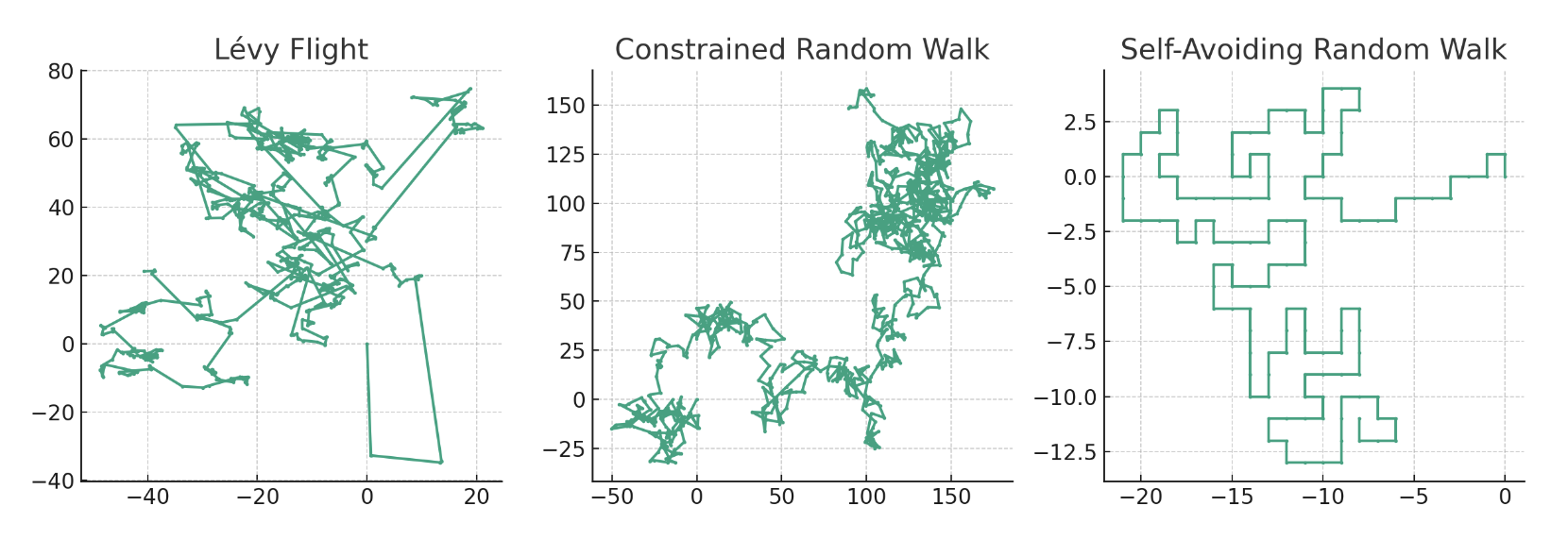
レヴィフライト(左)は長い距離をランダムに移動することが特徴です。このプロットでは、いくつかの非常に長いジャンプが見られます。

制約付きランダムウォーク(中)は移動距離に上限が設けられています。このプロットでは、各ステップの距離が一定の範囲内に収まっていることがわかります。

自己回避ランダムウォーク(右)は既に訪れた場所を避けるため、より複雑なパターンを形成しています。プロットでは、ルートが交差しないように進んでいるのが分かります。

プロット用のコード

import numpy as np
import matplotlib.pyplot as plt

# パラメータの設定
n_steps = 1000
step_size = 1

# 1. レヴィフライト
levy_exponent = 1.5
x_levy, y_levy = 0, 0
x_positions_levy, y_positions_levy = [x_levy], [y_levy]

for _ in range(n_steps):
    angle = np.random.uniform(0, 2 * np.pi)
    distance = np.random.pareto(levy_exponent)
    x_levy += distance * np.cos(angle)
    y_levy += distance * np.sin(angle)
    x_positions_levy.append(x_levy)
    y_positions_levy.append(y_levy)

# 2. 制約付きランダムウォーク
max_distance = 10
x_constrained, y_constrained = 0, 0
x_positions_constrained, y_positions_constrained = [x_constrained], [y_constrained]

for _ in range(n_steps):
    angle = np.random.uniform(0, 2 * np.pi)
    distance = np.random.uniform(0, max_distance)
    x_constrained += distance * np.cos(angle)
    y_constrained += distance * np.sin(angle)
    x_positions_constrained.append(x_constrained)
    y_positions_constrained.append(y_constrained)

# 3. 自己回避ランダムウォーク
x_self_avoiding, y_self_avoiding = 0, 0
x_positions_self_avoiding, y_positions_self_avoiding = [x_self_avoiding], [y_self_avoiding]
visited_positions = {(x_self_avoiding, y_self_avoiding)}

for _ in range(n_steps):
    possible_steps = []
    for dx, dy in [(1, 0), (-1, 0), (0, 1), (0, -1)]:
        new_pos = (x_self_avoiding + dx, y_self_avoiding + dy)
        if new_pos not in visited_positions:
            possible_steps.append(new_pos)
    
    if possible_steps:
        x_self_avoiding, y_self_avoiding = possible_steps[np.random.randint(len(possible_steps))]
        visited_positions.add((x_self_avoiding, y_self_avoiding))
        x_positions_self_avoiding.append(x_self_avoiding)
        y_positions_self_avoiding.append(y_self_avoiding)

# プロット
plt.figure(figsize=(12, 4))

# レヴィフライトのプロット
plt.subplot(1, 3, 1)
plt.plot(x_positions_levy, y_positions_levy, '-o', markersize=2)
plt.title('Lévy Flight')

# 制約付きランダムウォークのプロット
plt.subplot(1, 3, 2)
plt.plot(x_positions_constrained, y_positions_constrained, '-o', markersize=2)
plt.title('Constrained Random Walk')

# 自己回避ランダムウォークのプロット
plt.subplot(1, 3, 3)
plt.plot(x_positions_self_avoiding, y_positions_self_avoiding, '-o', markersize=2)
plt.title('Self-Avoiding Random Walk')

plt.tight_layout()
plt.show()

さいごに

ここまで基本的なランダム・ウォークの考え方、その派生形についてを学びました。

今後は「ランダムウォークを記述できることを活かした」"なにか"を考えてみたいと思います。

これは情報空間での探索過程においてランダムウォークからレヴィフライトへの移行が臨界点近くで発生し、大きなダイナミックレンジと高い柔軟性を持つという仮定したうえで、探索効率を最適化する計算方法を考えるものです。

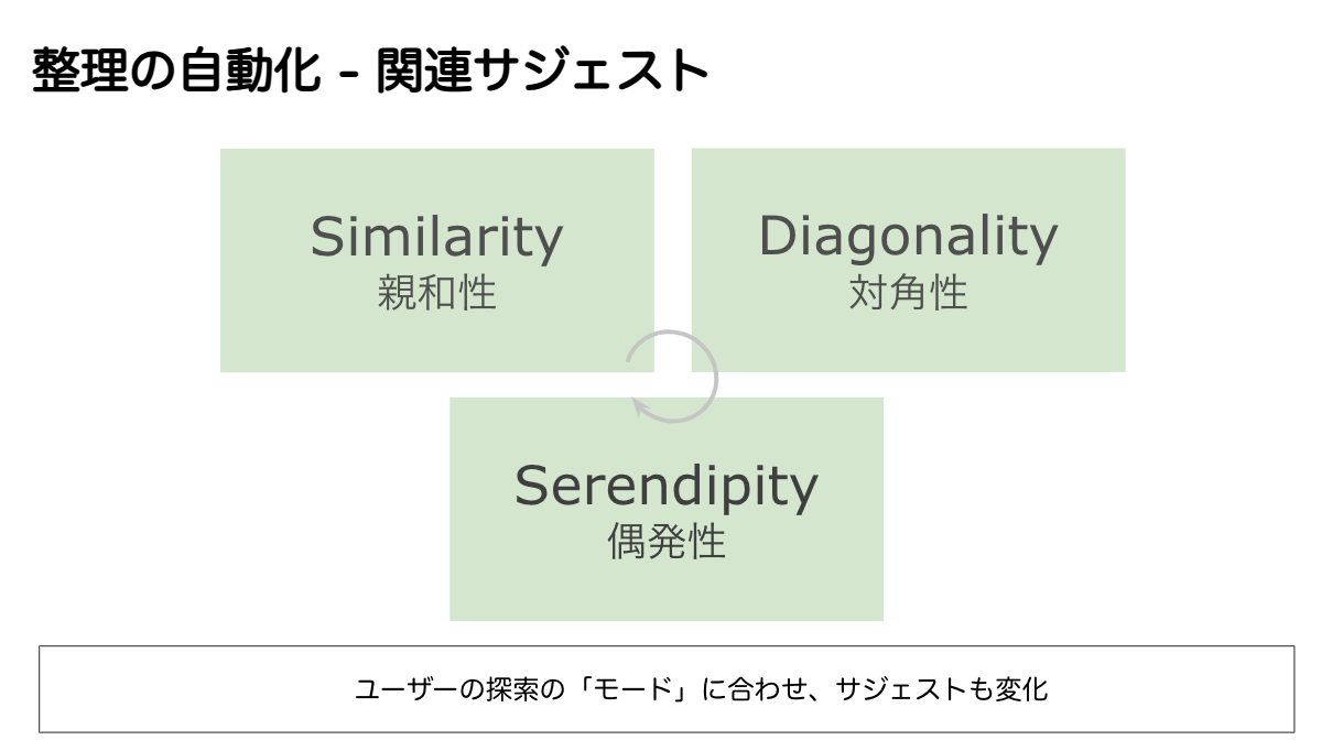
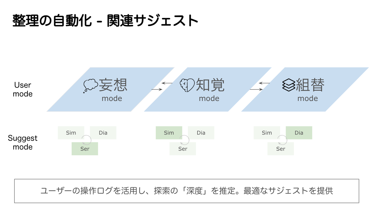
情報空間上の探索過程を、適応戦略としてどの段階にあるのかを把握し、サジェスチョンモードを切り替えるドキュメントシステムが実現できる形を考えていきたいと思います。

参考

臨界点付近で現れるレヴィーウォークの機能的利点 Masato S. Abe