さて、今回はD-wave(Leap)のOnline Learningで紹介されている、制限付きボルツマンマシン(RBM)のトレーニングに量子コンピュータ(D-wave)をする方法について書きます。
0 サンプルコード(ノートブック)の場所
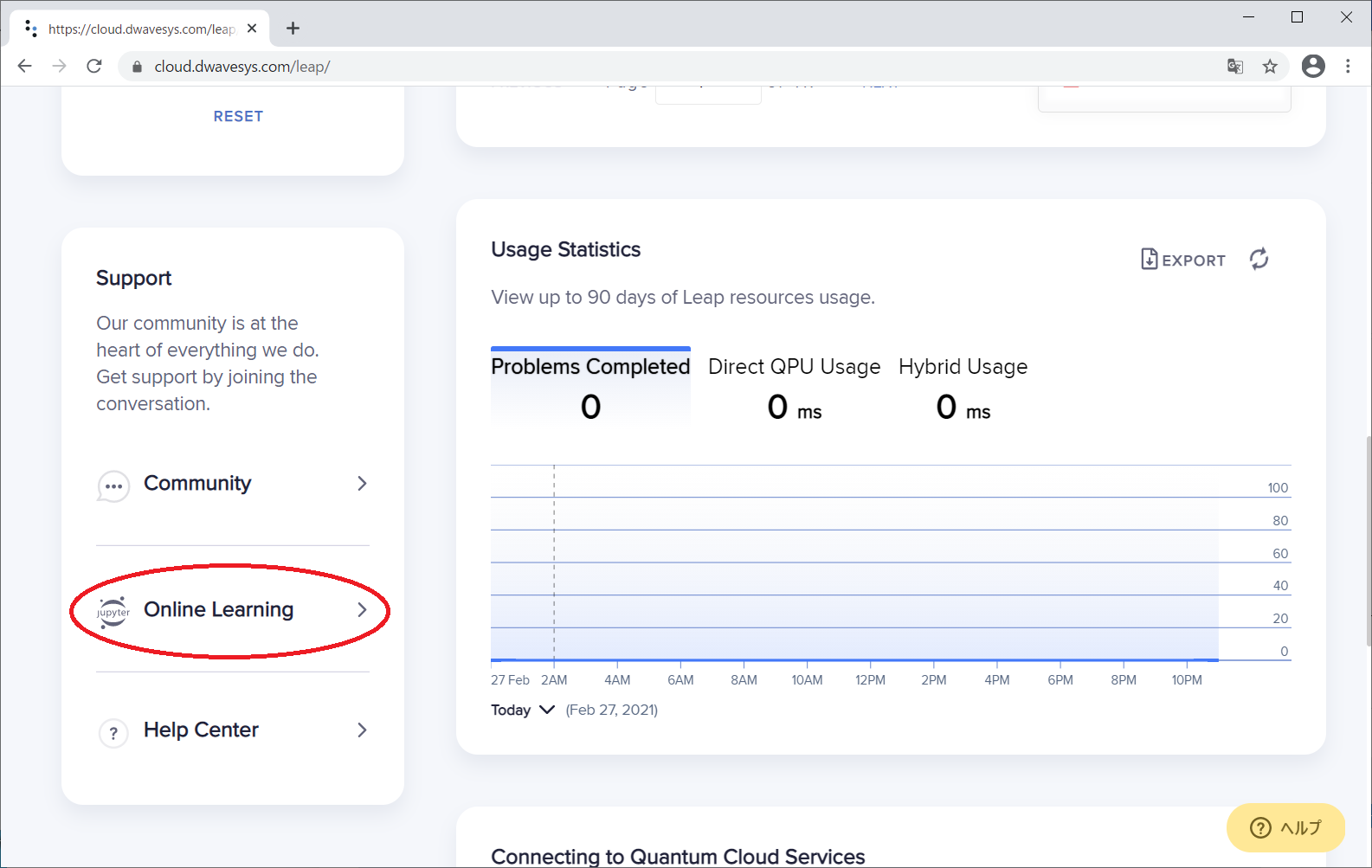
D-wave(Leap)にログインして、下方にスクロールすると左側に「Online Learning」というリンクが見えますので、これをクリックします。
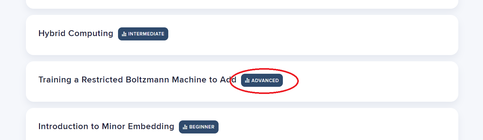
遷移先の画面で、下方にスクロールすると、「Training a Restricted Boltzmann Machine to Add」と表示されますので、これをクリックします。
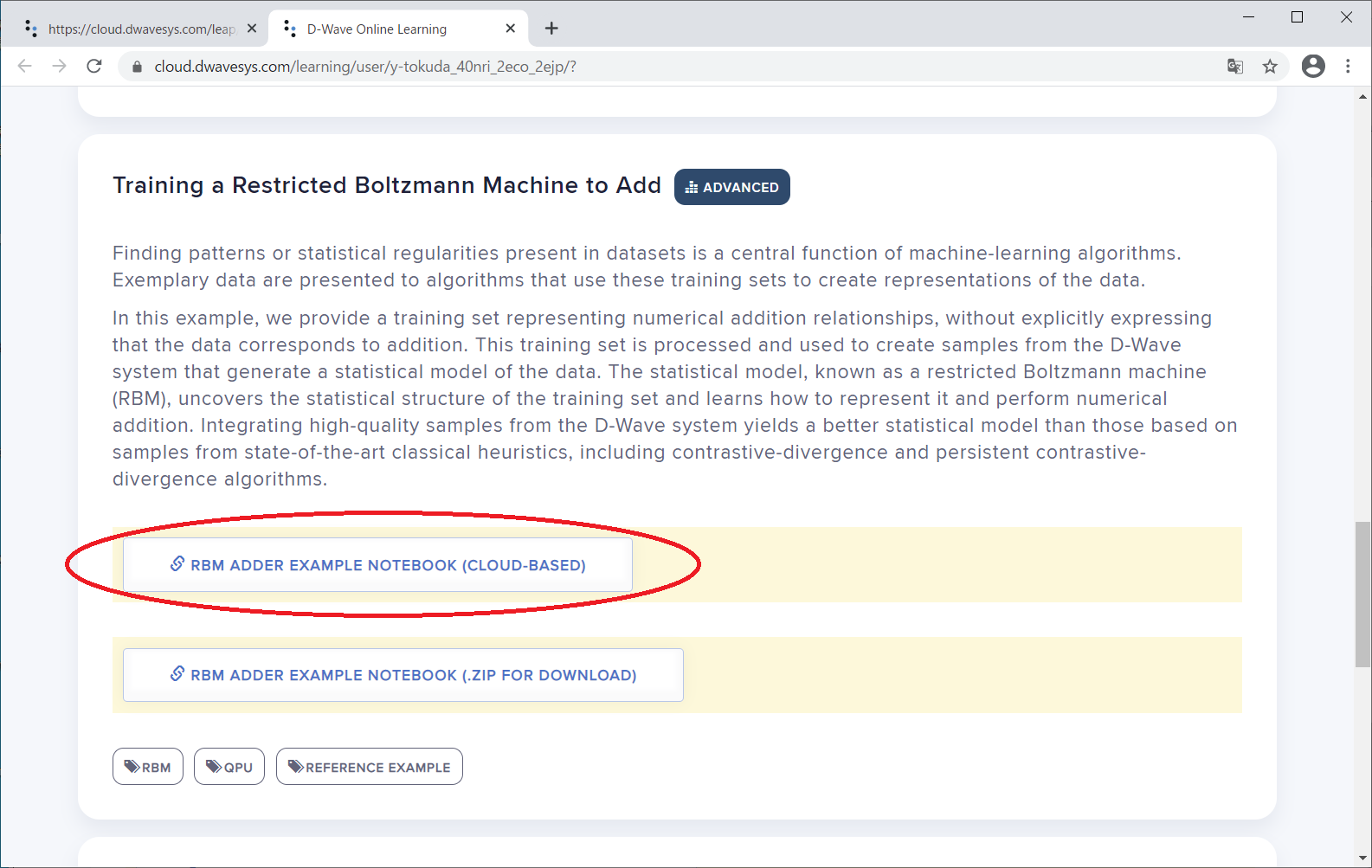
するとページが展開されるので、「RBM ADDER EXAMPLE NOTEBOOk(CLOUD-BASED)をクリックします。
すると、このように制限付きボルツマンマシンのサンプルNotebookが表示されます。これに記載されている内容を読んで行きます。
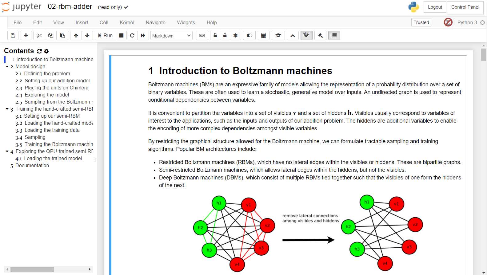
1. Introduction to Boltzmann machines
ボルツマンマシンの概要について解説している章です。。
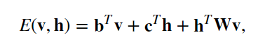
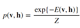
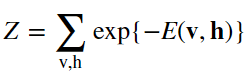
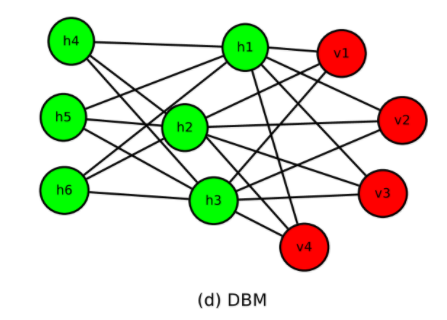
下記のような図で、ボルツマンマシン(BM)、制限付きボルツマンマシン(RBM)、semi-RBM、深層ボルツマンマシン(DBM)のについて説明しています。
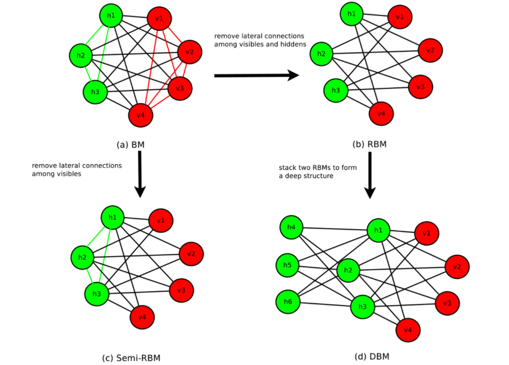
上記図中の、緑のユニットは、隠れユニット、赤色のユニットは可視ユニットです。ボルツマンマシン(BM)では、隠れユニットおよび可視ユニットのすべてが総合に接続されていますが、制限付きボルツマンマシン(RBM)では、可視ユニット同士、隠れユニット同士は接続されません。Semi-RBMでは、隠れユニット同士の相互に接続されますが、可視ユニット同士は接続されません。深層ボルツマンマシン(DBM)においては、隠れユニットが複数の層を構成しています。
隠れユニットをh、可視ユニットをvとすると、エネルギーが
で定義されること、および、確率分布は、
となることおよび、確率分布の式の分母Zは、分配関数
であることが、説明されています。
2 Model design
この章では、2つの3bitの2進数の加算を行うモデルを、RBMで作成するということを説明しています。入力としては、二つの3bitの2進数なので、6bit、出力としては、二つの3bitの加算結果なので、4bitを割り当てる旨が書かれています。キネマグラフ上、どのようにユニットが割り当てられるのかは、以下のように図示されています。
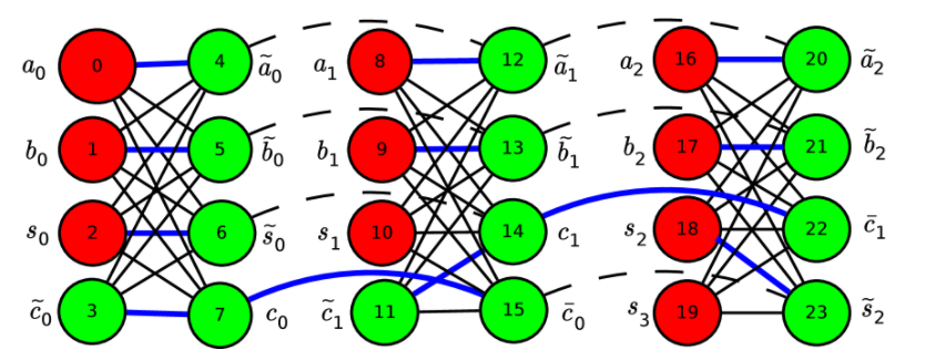
$a$と$b$は、加算対象の2進数(3bit)です。Sが加算結果の2進数(4bit)です。この図と対応する2進数の加算も記載されています。
そして、ボルツマンマシンを定義するコードがその下に記載されています。
from dwave_bm.rbm import BM

# Model dimensions.
num_visible = 10
num_hidden = [9, 5] # the hidden layer is a bipartite graph of 9 by 5

# Create the Boltzmann machine object
r = BM(num_visible=num_visible, num_hidden=num_hidden)
r
dwave.bm.rbmにBMというクラスが存在し、可視ユニット数と、隠れユニット数を与えるだけで、インスタンスを作れる様です。そして、このボルツマンマシン(semi-RBM)のエネルギーは次の式で与えられます。
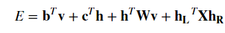
hとvはそれぞれ、可視ユニットおよび隠れユニットのビットを表現しているベクトルです。上式のうち、
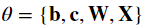
が、学習して決定するパラメタです。
どうやら、隠れユニットが2部グラフになっているパターンRBMのようです。Introductionでは、(d)として紹介されていた形ですね。
そして、下記のコードで、これらパラメータのshapeを確認できます。
# Dimensions

# Bias vector to visibles
print("b: {}".format(r.b_vect.shape))

# Bias vector to hiddens
print("c: {}".format(r.c_vect.shape))

# Weights between visibles and hiddens
print("W: {}".format(r.weights.shape))

# Lateral connections in hidden layer
print("X: {}".format(r.X.shape))
パラメータはまだトレーニングされていないので、まだ、3bitと3bitを加算する挙動はまったく期待できない状況ですが、とりあえずこのボルツマンマシンから5個、サンプリングしてみます。以下のコードです。
# Do not clamp any bits
clamped_bits = []

# Draw the samples
samples = r.sample_clamped_model(clamped_bits)

print "Obtained {} samples. The first 5 samples are:".format(len(samples))
print samples[0:5,:]
そして、サンプリングした値に対して、平均や標準偏差を計算してみます。次のコードです。
import numpy as np

N = len(samples)

# Calculate the mean of each variable by summing rows
means = sum([samples[i,:] for i in range(N)]) / float(N)

# Calculate the standard deviation of each variable
# with the row of means calculated above
stddevs = np.sqrt(sum([(samples[i,:] - means)**2 for i in range(N)]) / float(N))

print "means = {}".format(means)
まだトレーニングしていないので、平均は0.5付近、標準偏差も0.5程度です。
3 Training the hand-crafted semi-RBM with the QPU
これから、RBMをトレーニングします。まず、rbm_configs.jsonを作成します。rbm_configs.jsonには「D-wave leapのurl」、「接続の為のトークン」、「ソルバー名」を入れるようです。、下記のコードを見ると、tokenとsolver_nameは空になっているので、個々に、自身のtokenと、使用するソルバーの名前を入れなければいけない様子です。
# JSON config file with hardware credentials
# and structural information
import json
import os
hw_config_file_sample = 'rbm_configs.json'

# Set location for the configuration file to current working directory (CWD), if writeable, or /tmp/
write_base_path = os.getcwd()
if not os.access(write_base_path, os.W_OK):
    write_base_path='/tmp/'
hw_config_file = os.path.join(write_base_path, 'rbm_configs_example.json')

# define url, token and solver_name for running jobs on the hardware
url = 'https://cloud.dwavesys.com/sapi'
token = ''
solver_name = ''

with open(hw_config_file_sample, 'r') as cf:
    hw_config = json.load(cf)

# overwrite url, token and solver_name in the config
hw_config['url'] = url
hw_config['token'] = token
hw_config['solver'] = solver_name

# save to a new json file
with open(hw_config_file, 'w') as cf:
    json.dump(hw_config, cf, indent=4)

# print the config file
with open(hw_config_file, 'r') as cf:
    for line in cf.readlines():
        print line
そして、次のコードで、BMに対応するQuboファイルをロードします。原文で、下記コードの解説として「Here we load the model we designed earlier. 」と書いてあるのですが、このノートブックで実行したセルの中に、qubo-sample.txtを出力するようなコードは見当たりませんでした。というわけで、qubo-sample.txtはこのノートブックの為に、あらかじめ準備してあったサンプルかなと思われます。
# The file storing the designed model
model_file = 'dwave_bm/dimacs/qubo-sample.txt'

# Since the model was designed to fit into the native QPU graph,
# we use the BMPlacer class to load the problem graph.
from dwave_bm.rbm import BM, BMPlacer
placer = BMPlacer(num_visible, num_hidden, json_file=hw_config_file)
model = placer.read_model_dimacs_qubo(model_file)
BMPlacerのread_modelで取得した変数modelを引数にして、次のようにBMクラスのインスタンスを生成します。
# Create our BM object and pass it the designed model
r = BM(num_visible=num_visible, num_hidden=num_hidden,
       W_mask=placer.W_mask, X_mask=placer.X_mask,
       model=model)
次に、トレーニング用データをロードします。
m = np.load('dwave_bm/data/3-3-4.npz')
data_pos = m['data_pos']

data_pos = data_pos[np.random.permutation(data_pos.shape[0])]
そして、サンプラーとして'hw'(D-waveのハードウェアを使用するという意味と思われます)を指定します。
# Valid samplers are 'cd-10', 'pcd-10', 'hw'
sampler = 'hw'
そして、トレーニングの実行前に、以下のようにロガーを設定します。
# Function subscribe_logger writes the state of the BM out to
# disk (perhaps when )
from dwave_bm.example_utils import subscribe_logger

save_model = True
save_fig = False
# define a folder to save your result
result_folder = '/tmp/results/test_' + sampler

subscribe_logger(r, result_folder)

# This is how often we want to run the logger.
log_frequency = 10
そして、トレーニングの為のハイパーパラメータを設定します。
サンプリングにD-waveを使うだけなので、普通にボルツマンマシンをトレーニングするときと同様にハイパーパラメータが存在することがわかります。
# The maximum number of epochs to train.
# epochs = 10001
epochs = 101

# Minibatch size and number of samples are used to estimate the
# gradient of the cost function.
minibatch_size = 64

# Learning rate and momentum are used to calculate the next point
# \theta after the gradient is known.
eta0 = 0.5
learning_rate = [eta0*(1 / (1 + i / 200.0)) for i in range(epochs)]
momentum = 0.5
そしていよいよトレーニングです。が、下記のように全部コメントアウトされています!?
# Train the BM. Takes some time.
# Uncomment the following code to train your BM on the D-Wave quantum computer when it is necessary
# For debug purpose, try using `cd` or `pcd` as the sampler

# r.train(data_pos,
#         minibatch_size=minibatch_size,
#         max_epochs=epochs,
#         learning_rate=learning_rate,
#         momentum=momentum,
#         sampler=sampler,
#         part_l=placer.part_l,
#         part_r=placer.part_r,
#         save_model=save_model,
#         save_fig=save_fig,
#         hw_config_file=hw_config_file,
#         every_n_epochs=log_frequency,
#         )
よく見ると、このコードの上に、「とても時間がかかるから、やるときは慎重に!」と、ちょっと嫌なメッセージが書いてあります。もしかして実行するととてもお金がかかったりするのかも・・・

もしこの警告に怯まず、仮に実行したとすると、実行したノートブックのインスタンス上にボルツマンマシンのモデルのファイルが保存されます。そして、それはトレーニング完了後、下記のコードでロードできます。
# Some boilerplate to set up the environment
%matplotlib inline

sampler = 'hw'
# The directory in which to look for results.
# To use pre-generated results, set result_folder variable to 'results/hw'
result_folder = '/tmp/results/test_' + sampler

# A function to load the model saved during our previous training run
def load_model(epoch):
    from dwave_bm.example_utils import result_filename
    fn, result_epoch = result_filename(directory=result_folder,
                                       num_visible=num_visible,
                                       num_hidden=num_hidden,
                                       epoch=epoch,
                                       sampler=sampler
                                      )
    print "Loading model from '{}' for epoch '{}'".format(fn, result_epoch)
    return np.load(fn)

# The result epoch we would like to investigate
result_epoch = 'latest'

# We use the function defined above to load a model
m = load_model(result_epoch)

# The model is a numpy archive, which has several 'files' that
# parametrize the trained BM and some metadata
m.files
4 Exploring the QPU-trained semi-RBM
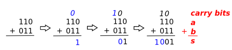
意図したようにトレーニングできたならば、このボルツマンマシンは、3bitの変数と3bitの変数を加算して、4bitの答えを出せる筈です。「加算できる」とはどういうことかと言うと、(v0,v1,v2)が、3bitの入力値、(v3,v4,v5)がもう一つ入力値なので、これらの値を固定した場合の(v6,v7,v8,v9)の値の確率分布が、二つの入力値の和のところが最大となるようになっているということです。つまり、

は、ちゃんと、sが、a+bの値のところが最大となっているということです。
ノートブックに記載されている内容によれば、下記のコードで確認できる筈です。
# Create a BM from a model saved in a previous training session
def load_BM(epoch=None):
    from dwave_bm.rbm import BM

    # Load the saved model, using function defined above
    m = load_model(epoch)

    # Create a BM object seeded with the loaded model
    return BM(num_visible=num_visible, num_hidden=num_hidden, model=m)


# Sample from the passed BM, clamping the inputs
def sample_clamped_inputs(  r,              # The BM to sample from
                            a = [1, 0, 1],  # a = 5 by default
                            b = [0, 1, 1],  # b = 3 by default
                          ):

    # Gather the clamps. The inputs are arranged with a first, then b,
    # in the order of visibles.
    clamped_bits = a + b

    # We can now sample from the clamped model.
    samples = r.sample_clamped_model(clamped_bits)

    # Show off some of the samples we got
    print "Obtained {} samples. The first 5 samples are:".format(len(samples))
    print samples[0:5, :]

    # For binary to int conversion
    from dwave_bm.example_utils import b2d

    # Find the correct answer from the integer values represented
    # by the clamped visible inputs
    correct_s = b2d(a) + b2d(b)

    # Count the number of samples that corresponded to the correct answer
    hits = map(b2d, samples).count(correct_s)

    # Print out the hit rate
    print "A total of {}/{} samples gave the correct answer.".format(hits, len(samples))

    return samples

# Now that we have some convenient ways of loading and sampling
# BMs, we can start out by loading the BM we had at the end
# of our previous training session.
r_trained = load_BM('latest')

# Here we set the values to which to clamp the inputs
a = [1, 0, 1]  # a = 5
b = [0, 1, 1]  # b = 3

# We can then draw some samples from it.
samples_trained = sample_clamped_inputs(r_trained, a=a, b=b)
ノートブック中の「とても時間がかかる」という警告は気になるのですが、同時にとても結果を見たいので、意を決して、実行してみたところ・・・残念ながら、以下のように最初のセルでいきなりエラーとなりました。
どうやら、このサンプルはPython2時代のもので、メンテされていないようです。D-wave leap上のnotebookで動かすことができないので、EC2に、Python2の環境を今更ながらですが作ってみて、チャレンジしてみようかなと思います。でもそもそもなんでこのサンプルメンテされてないんだろ?面白い応用例だと思うんですが。