多峰性をSilvermanの検定で確かめる

多峰性とは

ヒストグラムを作ったときに、よく山が複数できることがあります。これを多峰性(multimodal)と呼びます。
以下に、３つの正規分布を結合させて３つの山を持つデータをつくってみます。

# 正規分布を３つ結合させる。
x <- c(rnorm(100, mean = 4, sd = 1),
       rnorm(100, mean = 8, sd = 1),
       rnorm(100, mean = 12, sd = 1))

# 階級幅1でヒストグラムを描く。
hist(x, breaks=seq(0,16,1))

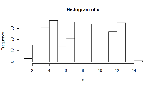
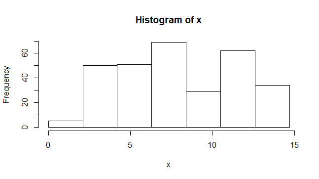
実際のデータでこの多峰性が現れた場合、データに複数の集団が含まれている可能性があります。しかし、ヒストグラムは階級幅の大きさによって形が変わってしまうため、本当の山(mode)の数はわかりません。例えば、先ほどのデータに対して階級幅を変えてヒストグラムを作ってみると、山の数が2個に見えるようになります。

# 階級幅2.1でヒストグラムを描く。
hist(x, breaks=seq(0,16,2.1))

この山の数を統計的な検定で決定したいと調べてみたところ、以下の資料に出会いました。

ノンパラメトリックな多峰性検定-Silvermanの検定-とその古生物学への導入

資料では、多峰性検定の一つであるSilvermanの検定をとてもわかりやすく説明しており、とても勉強になりました。Rのパッケージも紹介していたのですが、見つけることができなかったので、以下のパッケージを試してみました。

jenzoprさんのsilvermantestパッケージ（GitHub）

silvermantestパッケージの紹介

まず、導入してみます。

library(silvermantest)

silverman.testで検定を行うことができます。mode数が1のときは、キャリブレーションが必要となるので、adjust=TRUEとします。以下に、先ほどの３つの正規分布の結合データを検定してみました。

# mode数1で検定
silverman.test(x, 1, adjust = TRUE)

# mode数2で検定
silverman.test(x, 2)

# mode数3で検定
silverman.test(x, 3)

結果は以下のとおりです。mode数3でp値が0.05を超えました。mode数を3と考えて良さそうです。

Silvermantest: Testing the null hypothesis that the number of modes is <=  1 
The resulting p-value is  -4.5e-05 

Silvermantest: Testing the null hypothesis that the number of modes is <=  2 
The resulting p-value is  0.001001001 

Silvermantest: Testing the null hypothesis that the number of modes is <=  3 
The resulting p-value is  0.9479479 

Silvermantest: Testing the null hypothesis that the number of modes is <=  4 
The resulting p-value is  0.7767768 

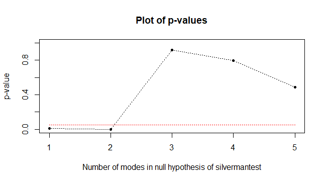
上記の操作をまとめて行えるのが、silverman.plotです。mode数ごとに検定を行って、p値をグラフにしてくれます。グラフの赤い線が0.05のラインです。p値が0.05を初めて超えたmode数を適切と考えてよいようです。

silverman.plot(x)

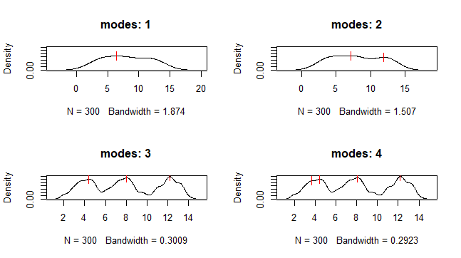
さらにdensities.plotで各mode数でのカーネル密度推定量のグラフを描くことができます。赤い線の部分が極大値を表しています。

densities.plot(x)

densities.plotのコードを加工して、ヒストグラムとカーネル密度推定量を重ねる関数を作ってみました。

# ヒストグラムとカーネル密度推定量を重ねる関数
hist_density = function(x, mode){

  # 極大値のインデックスを返す関数
  mode_ind = function(x, b) {
    y <- density(x, bw = b)$y
    d1 <- diff(y)
    signs <- diff(d1 / abs(d1))
    ind <- which(signs == -2)
    return(ind)
  }

  # 臨界バンド幅でのカーネル密度推定を行う。
  h0 <- h.crit(x, mode)
  d <- density(x, bw = h0)

  # グラフのx軸y軸の幅をを求める。
  y_max <- max(d$y)
  x_max <- max(abs(d$x))
  x_min <- min(abs(d$x))

  # カーネル密度推定量をプロット
  plot(d,
       main = paste("modes:", mode),
       xlim = c(x_min, x_max),
       ylim = c(0, y_max+0.1)
  )

  # 極大値のインデックスを求める。
  ind <- mode_ind(x, h0)

  x_values <- d$x
  y_values <- d$y

  # 極大値を赤くプロット。
  for (j in 1:mode){
    lines(c(x_values[ind[j]], x_values[ind[j]]),
          c(y_values[ind[j]] - 0.025, y_values[ind[j]] + 0.025),
          col = "red"
    )
  }

  # グラフを上書き。
  par(new=T)

  # ヒストグラムを描く
  hist(x,
       xlim = c(x_min, x_max),
       ylim = c(0, y_max+0.1),
       prob=T,
       ann=F)  

}

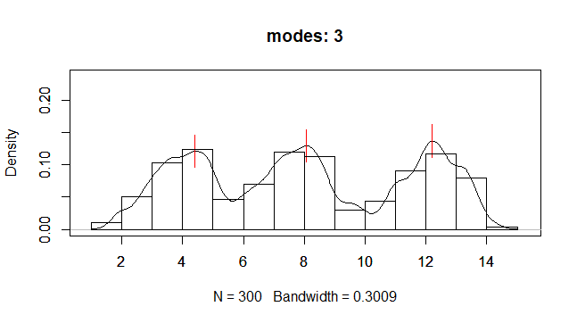
mode数3で実行してみます。

hist_density(x,3)

Rの多峰性に関するパッケージ

　今回はSilvermanの検定とパッケージについて紹介しましたが、他にも多峰性に関する検定はたくさんあります。また、CRANには多峰性に関するパッケージであるmultimodeがあり、多くの検定だけでなく、mode tree や mode forest 、SiZer map などを扱うことができます。