概要
前回の{tensorflow}を使ってみた記事を書いている最中に、importというPythonモジュールを読み込む関数を見つけて、試してみたら様々なモジュールが呼び出せたので忘れないように書いていく。今回はgensimによるHDP(Hierarchical Dirichlet Process)をやってみる。Rでの実行に対応するPythonスクリプトも一応残しておく。
はじめに
importを使うと何ができるようになるか簡単に説明すると、下記のようにPythonモジュールをRから呼び出して実行できる。
numpy <- tensorflow::import(module = "numpy")
# モジュール名にしなくてもOK(Pythonのimport XXX as YYYYで別名を与えるのと同じようなもの?)
pd <- tensorflow::import(module = "pandas")

# Numpyによる5行10列の乱数行列生成
> numpy$random$randn(5, 10)
           [,1]       [,2]        [,3]       [,4]       [,5]       [,6]       [,7]       [,8]       [,9]      [,10]
[1,]  0.2047579  1.4396232  1.39649920 -0.1621329 -0.6799612 -1.4375955  0.2590723 -1.4437292  1.1271664 -0.4434576
[2,] -0.3361488  0.5803642  0.95495572  0.6387092  0.6780120 -1.4093077 -1.3109703 -0.3436415 -0.3865685  1.7751260
[3,] -1.5810281 -1.2563752  0.89171330  0.6231667 -0.2083092 -0.3420242  0.3497256 -0.1856578  0.7441822  0.3541081
[4,]  0.8735340  1.3249083 -0.85038554  1.7963186 -0.4585773  0.8976184 -1.3661424  1.1888050 -1.0010572 -1.0871089
[5,] -0.5713605  0.6925751 -0.04234618  1.6234901  0.2355078 -0.2883208  1.6499782  1.6002583 -0.4482790 -0.0950429

# Pandasによるデータフレーム化
> pd$DataFrame(data = numpy$array(c(1, 2)))
     0
0  1.0
1  2.0
以前に書いた記事でRStudioの1系Preview版では{tensorflow}を呼び出すとTensorFlowのオブジェクトがサジェストされる旨に触れたが、importで呼び出したモジュールも同じように対応している。
下記の画像では上記で呼び出したPandasを例にしている。Pandasを読み込んだpdオブジェクトに$をつけてタブを押すと、関数やオブジェクトがサジェストされる。

これによりPythonに馴染みがないRStudioユーザーでも便利なモジュールが簡単に使えてしまう。なお、Pythonでは.でメソッドを呼び出すが、R上で呼び出す際には$を使うため、GitHubなどのPythonスクリプトをRで書き直す際には注意が必要になる。
辞書型の扱い方
話題がそれてしまうが、RにはPythonの辞書型がなくtensorflow::dictで作成した辞書オブジェクトの扱いに戸惑ったので、メモとして残しておく。
# 作成はtensorflow::dict()
> (word_dict <- tensorflow::dict(a = "at"))
{'a': 'at'}
> class(x = word_dict)
[1] "tensorflow.builtin.dict"   "tensorflow.builtin.object" "externalptr"

# 値の参照はget()メソッドを利用
> word_dict$get("a")
[1] "at"

# 存在しないキーを指定すると何も返さないので、判定ではis.null()を使う
> word_dict$get("b")
> is.null(x = word_dict$get("b"))
[1] TRUE
なお、RとPython間のオブジェクトの対応は{tensorflow}のAPIリファレンスが参考になる。
|Python|R|Examples|
|---|---|---|---|
|Scalar|Single-element vector|1, 1L, TRUE, "foo"|
|List|Multi-element vector|c(1.0, 2.0, 3.0), c(1L, 2L, 3L)|
|Tuple|List of multiple types|list(1L, TRUE, "foo")|
|Dict|Named list or dict|list(a = 1L, b = 2.0), dict(x = x_data)|
|NumPy ndarray|Matrix/Array|matrix(c(1,2,3,4), nrow = 2, ncol = 2)|
|None, True, False|NULL, TRUE, FALSE|NULL, TRUE, FALSE|
定義・設定
本題のgensimを使ったHDPの実行用の関数定義。もちろん、あらかじめgensimはインストールしておく必要がある。
library(pacman)

# 読み込むパッケージ
SET_LOAD_PACKAGE <- c("tensorflow", "dplyr", "tidyr", "tidytext", "tibble", "stringi", "ggplot2")
# hdpmodel.pyの__getitem__
# https://github.com/RaRe-Technologies/gensim/blob/master/gensim/models/hdpmodel.py
assignTopic <- function (hdp, corpus, eps = 0.01) {
  gamma <- hdp$inference(chunk = corpus)
  topic_dist <- gamma / matrix(data = rep(x = rowSums(x = gamma), hdp$m_T), ncol = hdp$m_T, byrow = FALSE)
  tpc_idx <- dplyr::as_data_frame(which(x = topic_dist >= eps, arr.ind = TRUE)) %>%
    dplyr::arrange(row, col)
  return(
    dplyr::data_frame(
      doc_id = tpc_idx$row,
      topic_number = tpc_idx$col - 1,
      prob = topic_dist[as.matrix(tpc_idx)]
    )
  )
}
準備
gensimのHDP実行に必要なRでのデータ整形を行う。途中経過を表示するので、Python実行と比較してほしい。
# 今回使用するパッケージを読み込み
pacman::p_load(char = SET_LOAD_PACKAGE, install = FALSE, character.only = TRUE)
# Pythonモジュールのgensimの読み込み
gensim <- tensorflow::import(module = "gensim")

# HDPにかけるテキスト
documents <-  c(
  "Human machine interface for lab abc computer applications",
  "A survey of user opinion of computer system response time",
  "The EPS user interface management system",
  "System and human system engineering testing of EPS",
  "Relation of user perceived response time to error measurement",
  "The generation of random binary unordered trees",
  "The intersection graph of paths in trees",
  "Graph minors IV Widths of trees and well quasi ordering",
  "Graph minors A survey"
)

> texts <- dplyr::data_frame(documents) %>%
  tibble::rownames_to_column(var = "sid") %>%
  tidytext::unnest_tokens(output = word, input = documents, token = "words") %>%
  dplyr::anti_join(
    y = dplyr::data_frame(word = c("for", "a", "of", "the", "and", "to", "in")),
    by = "word"
  ) %>%
  print
# A tibble: 52 × 2
     sid     word
   <chr>    <chr>
1      8 ordering
2      8    quasi
3      8     well
4      8   widths
5      8       iv
6      8   minors
7      9   minors
8      7    paths
9      7    graph
10     8    graph
# ... with 42 more rows

# gensim.corpora.Dictionaryで単語とIDを紐付けるオブジェクトを作成
dictionary <- gensim$corpora$Dictionary(list(stringi::stri_unique(str = texts$word)))
# 下記ではID = 0の単語が"minors"
> head(x = dictionary$token2id, n = 5)
$minors
[1] 0

$generation
[1] 1

$random
[1] 17

$iv
[1] 3

$engineering
[1] 4

> class(dictionary)
[1] "gensim.corpora.dictionary.Dictionary" "gensim.utils.SaveLoad"                "_abcoll.Mapping"
[4] "tensorflow.builtin.object"            "externalptr"

# doc2bowメソッドを適用できるように単語毎にlistに格納
# 文毎にlistがあり、単語毎にlistがある形
sentence <- texts %>%
  dplyr::group_by(sid) %>%
  dplyr::summarize(sentence = list(as.list(x = word))) %>%
  print
# A tibble: 9 × 2
    sid   sentence
  <chr>     <list>
1     1 <list [7]>
2     2 <list [7]>
3     3 <list [5]>
4     4 <list [6]>
5     5 <list [7]>
6     6 <list [5]>
7     7 <list [4]>
8     8 <list [8]>
9     9 <list [3]>

> sentence$sentence[[1]]
[[1]]
[1] "applications"

[[2]]
[1] "computer"

[[3]]
[1] "abc"

[[4]]
[1] "lab"

[[5]]
[1] "interface"

[[6]]
[1] "machine"

[[7]]
[1] "human"

# 各文毎にdoc2bowメソッドを適用してcorpusを作成
corpus <- lapply(X = sentence$sentence, FUN = dictionary$doc2bow)
Hierarchical Dirichlet Process
上記までで加工したcorpusを用いて、gensimのHDPを呼び出す。後述するが、ここではTopic数を150までで実行している。
hdp <- gensim$models$hdpmodel$HdpModel(corpus = corpus, id2word = dictionary, alpha = 1, T = 150L)

# show_topicsメソッドで作成したトピック上位100を取得
topic_most_words <- dplyr::bind_rows(
  lapply(
    X = hdp$show_topics(topics = -1L, topn = 100L, formatted = FALSE),
    FUN = function (topic_result) {
      return(
        dplyr::data_frame(
          topic_number = topic_result[[1]],
          word = sapply(X = topic_result[[2]], FUN = "[[", 1),
          weight = sapply(X = topic_result[[2]], FUN = "[[", 2)
        )
      )
    }
  )
)
# 各トピックでTOP1の重みの単語を出力
> topic_most_words %>%
  dplyr::group_by(topic_number) %>%
  dplyr::top_n(n = 1, wt = weight) %>%
  dplyr::glimpse()
Observations: 150
Variables: 3
$ topic_number <int> 0, 1, 2, 3, 4, 5, 6, 7, 8, 9, 10, 11, 12, 13, 14, 15, 16, 17, 18, 19, 20, 21, 22, 23, 24, 25, 26, 27, 28, 29, 30, 31, 3...
$ word         <chr> "iv", "abc", "machine", "opinion", "iv", "binary", "user", "time", "random", "unordered", "graph", "computer", "ordering"...
$ weight       <dbl> 0.12797694, 0.12662267, 0.14265295, 0.22422048, 0.07968149, 0.15725564, 0.12947385, 0.12292357, 0.12069854, 0.08766465,...

# トピック番号0の重みが上位10単語を表示
> topic_most_words %>%
  dplyr::filter(topic_number == 0) %>%
  dplyr::top_n(n = 10, wt = weight)
# A tibble: 10 × 3
   topic_number      word     weight
          <int>     <chr>      <dbl>
1             0        iv 0.12797694
2             0     error 0.09925327
3             0 unordered 0.08631031
4             0    widths 0.08567026
5             0      user 0.05359417
6             0 perceived 0.04646710
7             0     quasi 0.03670312
8             0    minors 0.03300030
9             0    survey 0.03216778
10            0  relation 0.03062379

# トピックの重みはトピック毎の合計が1.0になるように設定
> topic_most_words %>%
  dplyr::group_by(topic_number) %>%
  dplyr::summarize(sum_weight = sum(weight))
# A tibble: 150 × 2
   topic_number sum_weight
          <int>      <dbl>
1             0          1
2             1          1
3             2          1
4             3          1
5             4          1
6             5          1
7             6          1
8             7          1
9             8          1
10            9          1
# ... with 140 more rows

# Rで加工しない形は次の通り
> hdp$show_topics(topics = 1L, topn = 10L)
[1] "topic 0: 0.128*iv + 0.099*error + 0.086*unordered + 0.086*widths + 0.054*user + 0.046*perceived + 0.037*quasi + 0.033*minors + 0.032*survey + 0.031*relation"
トピック数について
HDP-LDAは明示的なトピック数を持たず、無限可変長のトピックを持つ。理論的には無限トピックだが、プログラム実行の都合上、あるトピック数までに定めることになる(前述の実行だと150までを設定)。無限可変長のトピックをパラメータによって打ち切り、結果として適したトピック数となるという認識ですが、間違っていたらすみません(勉強不足で申し訳ありません)。
# パラメータを変動させてトピックの割り当てを比較すると、ある程度の数で確率がほとんど0になるトピックが出てくる(適したトピック数は満遍なく確率が振られている状態と考えられる?)
> assignTopic(hdp = hdp, corpus = corpus, eps = 0.5) %>%
  tidyr::spread(key = topic_number, value = prob, fill = 0)
# A tibble: 7 × 4
  doc_id       `0`      `1`       `2`
*  <int>     <dbl>    <dbl>     <dbl>
1      2 0.0000000 0.000000 0.5794248
2      3 0.0000000 0.636553 0.0000000
3      4 0.0000000 0.549115 0.0000000
4      5 0.0000000 0.000000 0.6637392
5      7 0.8510308 0.000000 0.0000000
6      8 0.9171867 0.000000 0.0000000
7      9 0.8142352 0.000000 0.0000000

> assignTopic(hdp = hdp, corpus = corpus, eps = 0.05) %>%
  tidyr::spread(key = topic_number, value = prob, fill = 0)
# A tibble: 9 × 5
  doc_id       `0`       `1`       `2`       `3`
*  <int>     <dbl>     <dbl>     <dbl>     <dbl>
1      1 0.0000000 0.4434944 0.4689728 0.0000000
2      2 0.0000000 0.0000000 0.5794248 0.3236852
3      3 0.2711764 0.6365530 0.0000000 0.0000000
4      4 0.3718040 0.5491150 0.0000000 0.0000000
5      5 0.2609743 0.0000000 0.6637392 0.0000000
6      6 0.4543387 0.4534745 0.0000000 0.0000000
7      7 0.8510308 0.0000000 0.0000000 0.0000000
8      8 0.9171867 0.0000000 0.0000000 0.0000000
9      9 0.8142352 0.0000000 0.0000000 0.0000000

> assignTopic(hdp = hdp, corpus = corpus, eps = 0.005) %>%
  tidyr::spread(key = topic_number, value = prob, fill = 0)
# A tibble: 9 × 10
  doc_id        `0`        `1`        `2`        `3`         `4`         `5`         `6`         `7`         `8`
*  <int>      <dbl>      <dbl>      <dbl>      <dbl>       <dbl>       <dbl>       <dbl>       <dbl>       <dbl>
1      1 0.03606753 0.44349436 0.46897279 0.01310405 0.010056735 0.007288994 0.005646310 0.000000000 0.000000000
2      2 0.03447054 0.02405832 0.57942479 0.32368520 0.010056624 0.007288991 0.005646310 0.000000000 0.000000000
3      3 0.27117635 0.63655299 0.02365162 0.01747056 0.013409101 0.009718661 0.007528413 0.005514206 0.000000000
4      4 0.37180402 0.54911504 0.02026298 0.01497529 0.011494638 0.008330283 0.006452925 0.000000000 0.000000000
5      5 0.26097434 0.02382923 0.66373916 0.01309609 0.010056665 0.007288992 0.005646310 0.000000000 0.000000000
6      6 0.45433870 0.45347446 0.02357873 0.01746019 0.013408535 0.009718667 0.007528413 0.005514206 0.000000000
7      7 0.85103077 0.03833858 0.02829496 0.02095766 0.016090783 0.011662393 0.009034095 0.006617047 0.000000000
8      8 0.91718670 0.02139333 0.01567863 0.01164270 0.008939062 0.006479106 0.005018942 0.000000000 0.000000000
9      9 0.81423517 0.04750129 0.03534385 0.02619753 0.020113102 0.014577990 0.011292619 0.008271309 0.005930772


# 以下はeps = 0.01の結果で検証する
topic_assign <- assignTopic(hdp = hdp, corpus = corpus)
topic_assign %>%
  tidyr::spread(key = topic_number, value = prob, fill = 0)
# A tibble: 9 × 8
  doc_id        `0`        `1`        `2`        `3`        `4`        `5`        `6`
*  <int>      <dbl>      <dbl>      <dbl>      <dbl>      <dbl>      <dbl>      <dbl>
1      1 0.03606753 0.44349436 0.46897279 0.01310405 0.01005674 0.00000000 0.00000000
2      2 0.03447054 0.02405832 0.57942479 0.32368520 0.01005662 0.00000000 0.00000000
3      3 0.27117635 0.63655299 0.02365162 0.01747056 0.01340910 0.00000000 0.00000000
4      4 0.37180402 0.54911504 0.02026298 0.01497529 0.01149464 0.00000000 0.00000000
5      5 0.26097434 0.02382923 0.66373916 0.01309609 0.01005666 0.00000000 0.00000000
6      6 0.45433870 0.45347446 0.02357873 0.01746019 0.01340854 0.00000000 0.00000000
7      7 0.85103077 0.03833858 0.02829496 0.02095766 0.01609078 0.01166239 0.00000000
8      8 0.91718670 0.02139333 0.01567863 0.01164270 0.00000000 0.00000000 0.00000000
9      9 0.81423517 0.04750129 0.03534385 0.02619753 0.02011310 0.01457799 0.01129262

# 確率が最大となるトピック番号をトピックとして割り当てると、0から2までに集中
> topic_assign %>%
  dplyr::group_by(doc_id) %>%
  dplyr::filter(prob == max(prob))
Source: local data frame [9 x 3]
Groups: doc_id [9]

  doc_id topic_number      prob
   <int>        <dbl>     <dbl>
1      1            2 0.4689728
2      2            2 0.5794248
3      3            1 0.6365530
4      4            1 0.5491150
5      5            2 0.6637392
6      6            0 0.4543387
7      7            0 0.8510308
8      8            0 0.9171867
9      9            0 0.8142352

# トピック番号毎に比率を出す
> dplyr::left_join(
  x = topic_assign %>%
    dplyr::group_by(topic_number) %>%
    dplyr::summarize(topic_sum_prob = sum(prob)),
  y = topic_assign %>%
    dplyr::mutate(sum_prob = sum(prob)) %>%
    dplyr::distinct(topic_number, sum_prob),
  by = "topic_number"
) %>%
  dplyr::mutate(
    ratio = topic_sum_prob / sum_prob,
    cumsum_ratio = cumsum(x = ratio)
  ) %>%
  dplyr::select(topic_number, ratio, cumsum_ratio)
# A tibble: 7 × 3
  topic_number       ratio cumsum_ratio
         <dbl>       <dbl>        <dbl>
1            0 0.460601369    0.4606014
2            1 0.256953677    0.7175550
3            2 0.213456275    0.9310113
4            3 0.052658161    0.9836695
5            4 0.012020739    0.9956902
6            5 0.003013089    0.9987033
7            6 0.001296691    1.0000000
eps = 0.01のときは、トピック数が3から4くらいでほぼ網羅でき、多くても7までという結果だろうか。
可視化
トピック番号0から6までの7トピックに限定し、様々な切り口で可視化してみる。
トピック毎に単語の重み累積和を可視化
tpc_words <- dplyr::inner_join(
  x = topic_most_words,
  y = topic_assign %>%
    dplyr::distinct(topic_number),
  by = "topic_number"
)

tpc_words %>%
  dplyr::mutate(topic_number = as.factor(x = topic_number)) %>%
  dplyr::group_by(topic_number) %>%
  dplyr::mutate(
    counter = dplyr::row_number(x = topic_number),
    cumsum_weight = cumsum(x = weight)
  ) %>%
  ggplot2::ggplot(
    data = ., mapping = ggplot2::aes(x = counter, y = cumsum_weight)
  ) + ggplot2::geom_line(mapping = ggplot2::aes(group = topic_number, color = topic_number))
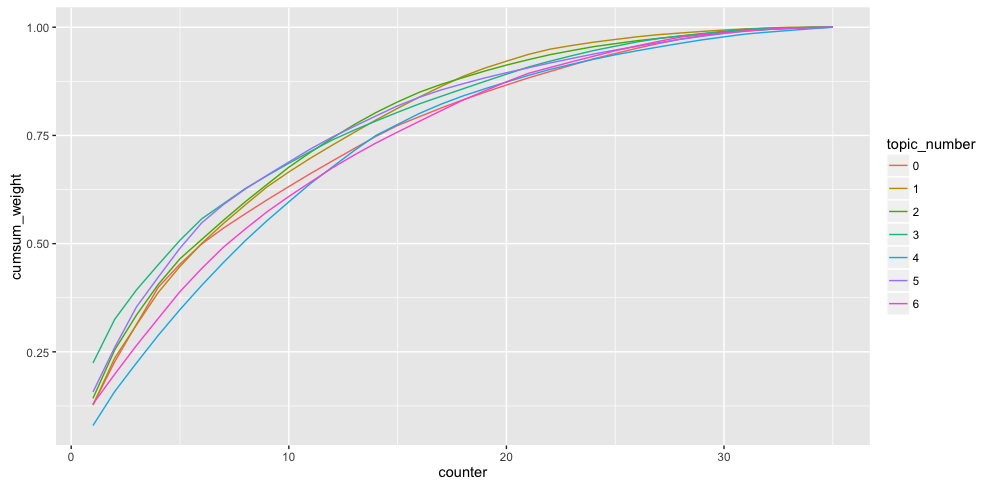
上位5単語のとき(X軸が5のライン)では、トピック番号3は約0.50でトピック番号4は約0.28となっており、トピック番号3の方が少ない単語に高い確率が付与されていることがわかる(いくつかの単語がトピック番号3を強く表現していると考えられる)。
トピック毎に重み上位10単語を可視化
tpc_words %>%
  dplyr::group_by(topic_number) %>%
  dplyr::arrange(topic_number, dplyr::desc(x = weight)) %>%
  dplyr::top_n(n = 10, wt = weight) %>%
  dplyr::mutate(word = reorder(x = word, X = weight)) %>%
  dplyr::ungroup() %>%
  ggplot2::ggplot(data = ., mapping = ggplot2::aes(x = word, y = weight, fill = factor(topic_number))) +
  ggplot2::geom_bar(stat = "identity", show.legend = FALSE) +
  ggplot2::facet_wrap(facets = ~ topic_number, scales = "free") +
  ggplot2::theme(axis.text.x = ggplot2::element_text(angle = 90))
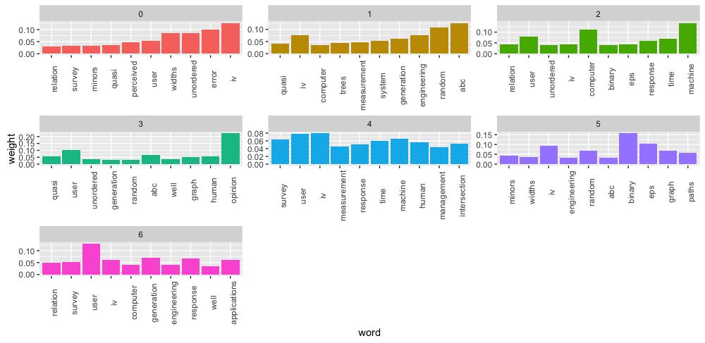
トピック番号3は"opinion"と"user"の割合が大きく、トピック番号4は単語毎に満遍なく重みが付与されている。これはひとつ前の可視化を単語レベルで確認しているとも。
トピック毎に重み上位30単語を単語毎に積み上げ棒グラフで可視化
tpc_words %>%
  dplyr::group_by(topic_number) %>%
  dplyr::arrange(topic_number, dplyr::desc(x = weight)) %>%
  dplyr::top_n(n = 30, wt = weight) %>%
  dplyr::ungroup() %>%
  dplyr::mutate(
    topic_number = factor(topic_number),
    word = reorder(x = word, X = weight)
  ) %>%
  ggplot2::ggplot(ggplot2::aes(x = word, y = weight, fill = topic_number)) +
  ggplot2::geom_bar(stat = "identity") + ggplot2::coord_flip()
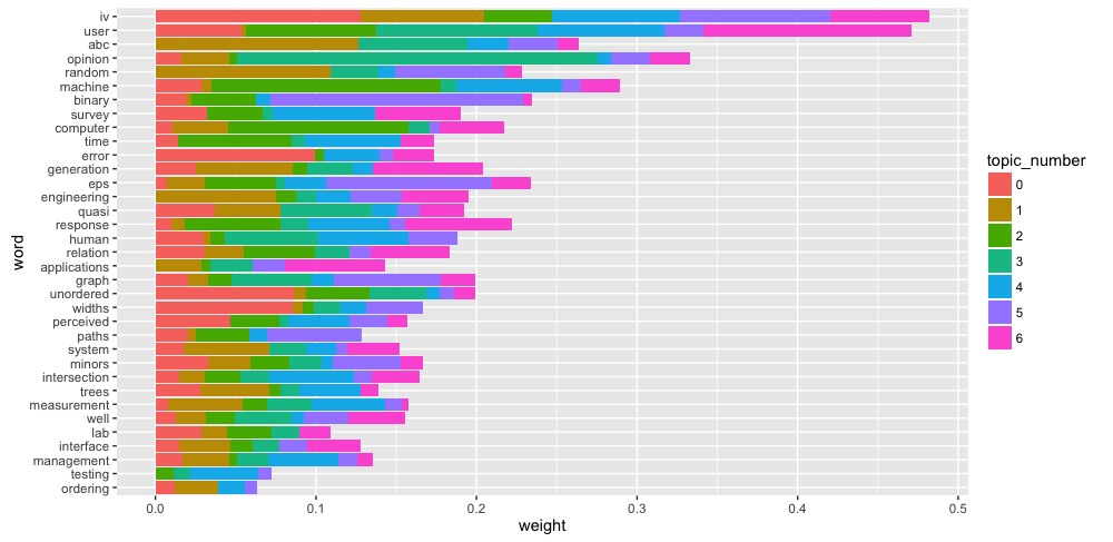
単語毎にトピックの割合が可視化できると考えられる。具体的には、"error"はトピック番号0に大きい割合を占め、"opinion"はひとつ前の可視化の結果通りトピック番号3の割合が大きい。対照的に、"iv"や"user"などはひとつのトピックに捉われないとも。
まとめ
{tensorflow}のimportというPythonモジュールを読み込む関数を用いて、gensimのHDPを実行しました。さらに適してそうなトピック数を求め、結果を様々な切り口で可視化してみました。HDPの知識が足らず、正しい認識かどうか心配ですが、とりあえずやってみました(ここがおかしいなどがありましたらが、ご指摘いただけると幸いです)。同じようにgensimのDoc2Vecも実行検証したので、そのうちまとめます。
{tensorflow}のimportで以前から愛用していた{PythonInR}を使わなくなるかと思ったのですが、Pythonでは呼び出せる関数が読み出せなかったりするので、もう少し調査したいです。
> gensim$models$ldaseqmodel$LdaSeqModel
 eval(substitute(expr), envir, enclos) でエラー:
  AttributeError: 'module' object has no attribute 'ldaseqmodel'
import gensim
>>> gensim.models.ldaseqmodel.LdaSeqModel
<class 'gensim.models.ldaseqmodel.LdaSeqModel'>
追記(2016.01.04)
上記のgensimでDTMが呼び出せない件について、tensorflowのバージョンを上げたところ利用できました(実行を確認できた環境は0.12.1)。ただし、pip install tensorflowではダメで、公式にある通りの手順でTF_BINARY_URLで.whlを指定するとできました。違いがよくわかりません。
dtm <- gensim$models$ldaseqmodel$LdaSeqModel(corpus = corpus, time_slice = c(5L, 10L, 15L), num_topics = 3L)
> print(dtm)
LdaSeqModel

# 指定した文書のトピック分布
> dtm$doc_topics(doc_number = 1)
[1] 0.001422475 0.001422475 0.997155050

# 文書毎のトピック分布、単語毎のトピック分布、文毎の単語数、単語毎の出現頻度
> dtm$dtm_vis(time = 1L, corpus = corpus)
[[1]]
             [,1]        [,2]        [,3]
 [1,] 0.001422475 0.001422475 0.997155050
 [2,] 0.001422475 0.001422475 0.997155050
 [3,] 0.001988072 0.001988072 0.996023857
 [4,] 0.001658375 0.001658375 0.996683250
 [5,] 0.001422475 0.001422475 0.997155050
 [6,] 0.996023857 0.001988072 0.001988072
 [7,] 0.995037221 0.002481390 0.002481390
 [8,] 0.001245330 0.997509340 0.001245330
 [9,] 0.003300330 0.993399340 0.003300330

[[2]]
           [,1]       [,2]       [,3]        [,4]       [,5]       [,6]       [,7]       [,8]
[1,] 0.05957456 0.01419498 0.01419498 0.014194979 0.01419498 0.01419498 0.01419498 0.01419498
[2,] 0.20229085 0.04711086 0.01035351 0.041352822 0.01035351 0.01035351 0.01035351 0.01035351
[3,] 0.01935312 0.01369708 0.01369708 0.007190831 0.01369708 0.07356165 0.01369708 0.07356165
           [,9]      [,10]       [,11]      [,12]       [,13]       [,14]      [,15]      [,16]
[1,] 0.01419498 0.01419498 0.128644022 0.01419498 0.014194979 0.128644022 0.01419498 0.01419498
[2,] 0.01035351 0.01035351 0.010353508 0.01035351 0.041352822 0.202290845 0.01035351 0.01035351
[3,] 0.01369708 0.01369708 0.007190831 0.01369708 0.007190831 0.007190831 0.13245925 0.01369708
           [,17]      [,18]      [,19]      [,20]      [,21]      [,22]      [,23]      [,24]
[1,] 0.014194979 0.01419498 0.01419498 0.01419498 0.12864402 0.01419498 0.01419498 0.01419498
[2,] 0.041352822 0.01035351 0.01035351 0.01035351 0.04135282 0.01035351 0.01035351 0.01035351
[3,] 0.007190831 0.01369708 0.01369708 0.01369708 0.01369708 0.01369708 0.01369708 0.01369708
          [,25]       [,26]      [,27]      [,28]       [,29]       [,30]      [,31]      [,32]
[1,] 0.01419498 0.128644022 0.01419498 0.01419498 0.014194979 0.014194979 0.01419498 0.01419498
[2,] 0.01035351 0.010353508 0.01035351 0.01035351 0.041352822 0.041352822 0.01035351 0.04135282
[3,] 0.07356165 0.007190831 0.07356165 0.01369708 0.007190831 0.007190831 0.07356165 0.01369708
          [,33]      [,34]      [,35]
[1,] 0.01419498 0.01419498 0.01419498
[2,] 0.01035351 0.01035351 0.01035351
[3,] 0.07356165 0.01369708 0.10274367

[[3]]
[1] 7 7 5 5 7 5 4 8 3

[[4]]
 [1] 2 1 1 1 1 2 1 2 1 1 1 1 1 3 4 1 1 1 1 1 3 1 1 1 2 1 2 1 1 1 2 2 2 1 3

[[5]]
 [1] "0"  "1"  "2"  "3"  "4"  "5"  "6"  "7"  "8"  "9"  "10" "11" "12" "13" "14" "15" "16" "17"
[19] "18" "19" "20" "21" "22" "23" "24" "25" "26" "27" "28" "29" "30" "31" "32" "33" "34"
参考
- 階層ディリクレ過程を実装してみる (1) HDP-LDA と LDA のモデルを比較
- GensimのHDP(Hierarchical Dirichlet Process)をクラシック音楽情報に対して試してみる
Pythonコード
HDPを呼び出しに使ったPythonスクリプト。
Python 2.7.12 (default, Jul 10 2016, 20:09:20)
[GCC 4.2.1 Compatible Apple LLVM 7.3.0 (clang-703.0.31)] on darwin
Type "help", "copyright", "credits" or "license" for more information.
import gensim
import pandas


# HDPにかけるテキスト
documents = ["Human machine interface for lab abc computer applications",
"A survey of user opinion of computer system response time",
"The EPS user interface management system",
"System and human system engineering testing of EPS",
"Relation of user perceived response time to error measurement",
"The generation of random binary unordered trees",
"The intersection graph of paths in trees",
"Graph minors IV Widths of trees and well quasi ordering",
"Graph minors A survey"]

# ストップワード定義
stoplist = set('for a of the and to in'.split())


# テキスト前処理
texts = [[word for word in document.lower().split() if word not in stoplist] for document in documents]
>>> pprint(texts)
[['human', 'machine', 'interface', 'lab', 'abc', 'computer', 'applications'],
 ['survey', 'user', 'opinion', 'computer', 'system', 'response', 'time'],
 ['eps', 'user', 'interface', 'management', 'system'],
 ['system', 'human', 'system', 'engineering', 'testing', 'eps'],
 ['relation', 'user', 'perceived', 'response', 'time', 'error', 'measurement'],
 ['generation', 'random', 'binary', 'unordered', 'trees'],
 ['intersection', 'graph', 'paths', 'trees'],
 ['graph', 'minors', 'iv', 'widths', 'trees', 'well', 'quasi', 'ordering'],
 ['graph', 'minors', 'survey']]

dictionary = gensim.corpora.Dictionary(texts)
>>> pprint(dictionary.token2id)
{u'abc': 0,
 u'applications': 3,
 u'binary': 22,
 u'computer': 4,
 u'engineering': 15,
 u'eps': 14,
 u'error': 18,
 u'generation': 21,
 u'graph': 26,
 u'human': 5,
 u'interface': 6,
 u'intersection': 27,
 u'iv': 33,
 u'lab': 1,
 u'machine': 2,
 u'management': 13,
 u'measurement': 20,
 u'minors': 29,
 u'opinion': 11,
 u'ordering': 30,
 u'paths': 28,
 u'perceived': 17,
 u'quasi': 34,
 u'random': 23,
 u'relation': 19,
 u'response': 12,
 u'survey': 8,
 u'system': 7,
 u'testing': 16,
 u'time': 10,
 u'trees': 25,
 u'unordered': 24,
 u'user': 9,
 u'well': 32,
 u'widths': 31}
corpus = [dictionary.doc2bow(text) for text in texts]
>>> pprint(corpus)
[[(0, 1), (1, 1), (2, 1), (3, 1), (4, 1), (5, 1), (6, 1)],
 [(4, 1), (7, 1), (8, 1), (9, 1), (10, 1), (11, 1), (12, 1)],
 [(6, 1), (7, 1), (9, 1), (13, 1), (14, 1)],
 [(5, 1), (7, 2), (14, 1), (15, 1), (16, 1)],
 [(9, 1), (10, 1), (12, 1), (17, 1), (18, 1), (19, 1), (20, 1)],
 [(21, 1), (22, 1), (23, 1), (24, 1), (25, 1)],
 [(25, 1), (26, 1), (27, 1), (28, 1)],
 [(25, 1), (26, 1), (29, 1), (30, 1), (31, 1), (32, 1), (33, 1), (34, 1)],
 [(8, 1), (26, 1), (29, 1)]]


# HDP実行
hdp = gensim.models.hdpmodel.HdpModel(corpus = corpus, id2word = dictionary, alpha = 1.0, T = 150)
pandas.DataFrame([dict(hdp[x]) for x in corpus])
          0         1         2         3         4         5        6
0  0.153961  0.024102  0.017490  0.013135  0.763441       NaN      NaN
1  0.424649  0.506962  0.017490  0.013132       NaN       NaN      NaN
2  0.234524  0.033107  0.664496  0.017517  0.013194       NaN      NaN
3  0.894362  0.027382  0.020088  0.015006  0.011309       NaN      NaN
4  0.907610  0.023981  0.017512  0.013130       NaN       NaN      NaN
5  0.052698  0.856097  0.023335  0.017514  0.013194       NaN      NaN
6  0.054569  0.835891  0.028101  0.021013  0.015832  0.011575      NaN
7  0.029701  0.478424  0.015533  0.011674       NaN  0.437527      NaN
8  0.066220  0.797049  0.034939  0.026260  0.019790  0.014469  0.01079
実行環境
Session info ----------------------------------------------------------------------------------------------------------------------
 setting  value
 version  R version 3.3.1 (2016-06-21)
 system   x86_64, darwin13.4.0
 ui       RStudio (1.0.44)
 language (EN)
 collate  ja_JP.UTF-8
 tz       Asia/Tokyo
 date     2016-10-30

Packages --------------------------------------------------------------------------------------------------------------------------
 package     * version date       source
 assertthat    0.1     2013-12-06 CRAN (R 3.3.1)
 broom         0.4.1   2016-06-24 CRAN (R 3.3.0)
 colorspace    1.2-6   2015-03-11 CRAN (R 3.3.1)
 DBI           0.5     2016-08-11 cran (@0.5)
 devtools      1.12.0  2016-06-24 CRAN (R 3.3.0)
 digest        0.6.9   2016-01-08 CRAN (R 3.3.0)
 dplyr       * 0.5.0   2016-06-24 CRAN (R 3.3.1)
 ggplot2     * 2.1.0   2016-03-01 CRAN (R 3.3.1)
 gtable        0.2.0   2016-02-26 CRAN (R 3.3.1)
 janeaustenr   0.1.1   2016-06-20 CRAN (R 3.3.0)
 lattice       0.20-33 2015-07-14 CRAN (R 3.3.1)
 magrittr      1.5     2014-11-22 CRAN (R 3.3.1)
 Matrix        1.2-6   2016-05-02 CRAN (R 3.3.1)
 memoise       1.0.0   2016-01-29 CRAN (R 3.3.0)
 mnormt        1.5-4   2016-03-09 CRAN (R 3.3.0)
 munsell       0.4.3   2016-02-13 CRAN (R 3.3.1)
 nlme          3.1-128 2016-05-10 CRAN (R 3.3.1)
 pacman      * 0.4.1   2016-03-30 CRAN (R 3.3.0)
 plyr          1.8.4   2016-06-08 CRAN (R 3.3.1)
 psych         1.6.6   2016-06-28 CRAN (R 3.3.0)
 R6            2.1.3   2016-08-19 cran (@2.1.3)
 Rcpp          0.12.7  2016-09-05 cran (@0.12.7)
 reshape2      1.4.1   2014-12-06 CRAN (R 3.3.1)
 scales        0.4.0   2016-02-26 CRAN (R 3.3.1)
 SnowballC     0.5.1   2014-08-09 CRAN (R 3.3.1)
 stringi     * 1.1.1   2016-05-27 CRAN (R 3.3.1)
 stringr       1.1.0   2016-08-19 cran (@1.1.0)
 tensorflow  * 0.3.0   2016-10-25 Github (rstudio/tensorflow@dfe2f1a)
 tibble      * 1.2     2016-08-26 cran (@1.2)
 tidyr       * 0.6.0   2016-08-12 cran (@0.6.0)
 tidytext    * 0.1.1   2016-06-25 CRAN (R 3.3.0)
 tokenizers    0.1.4   2016-08-29 CRAN (R 3.3.0)
 withr         1.0.2   2016-06-20 CRAN (R 3.3.0)