Open NGC カタログとは
OpenNGC とは、NGC (New General Catalogue) and IC (Index Catalogue)を整理したデータベースのこと。
ソースコードを見ればわかる人は、Google Colab を参照ください。
python インターフェースの PyOngc
https://github.com/mattiaverga/PyOngc を使うと、簡単にデータを取得することができる。python3系で pip install pyongc でインストールできる。
import pyongc
name="NGC4051"
DSOobject = pyongc.Dso(name)
gtype = DSOobject.getType()
mag = DSOobject.getMagnitudes()
surf = DSOobject.getSurfaceBrightness()
hubble = DSOobject.getHubble()
# print(gtype,mag,surf,hubble)
# ('Galaxy', (11.08, 12.92, 8.58, 8.06, 7.67), 22.87, 'SABb')
pyongcをインストールすると、コマンドラインツールもインストールされて、星や銀河がどのくらい含まれているかは次のコマンドでわかる。
> ongc stats

PyONGC version: 0.5.1
Database version: 20191019
Total number of objects in database: 13978
Object types statistics:
	Star                         -> 546
	Double star                  -> 246
	Association of stars         -> 62
	Star cluster + Nebula        -> 66
	Dark Nebula                  -> 2
	Duplicated record            -> 636
	Emission Nebula              -> 8
	Galaxy                       -> 10490
	Globular Cluster             -> 205
	Group of galaxies            -> 16
	Galaxy Pair                  -> 212
	Galaxy Triplet               -> 23
	HII Ionized region           -> 83
	Nebula                       -> 93
	Nonexistent object           -> 14
	Nova star                    -> 3
	Open Cluster                 -> 661
	Object of other/unknown type -> 434
	Planetary Nebula             -> 129
	Reflection Nebula            -> 38
	Supernova remnant            -> 11
全カタログを解析する場合
全部のカタログを解析したい場合は、大元のcsvファイルをダウンロードしてしまいましょう。wgetがインストールされている場合は下記で一発でダウンロードできるはず。
wget https://raw.githubusercontent.com/mattiaverga/OpenNGC/master/NGC.csv .
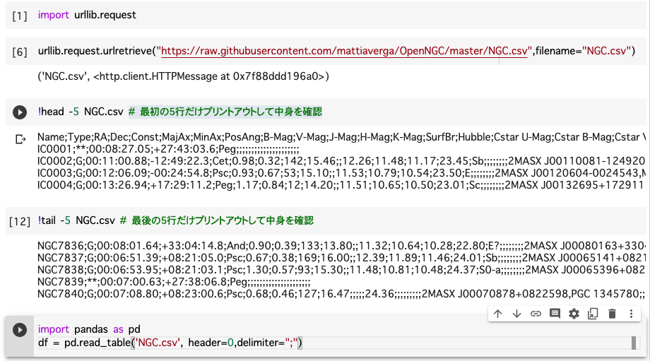
あるいは、urllib.request.urlretrieve を使っても、
import urllib.request
urllib.request.urlretrieve("https://raw.githubusercontent.com/mattiaverga/OpenNGC/master/NGC.csv",filename="NGC.csv")
で1発でファイルに保存してくれます。私の Google Colab だと次のようになります。
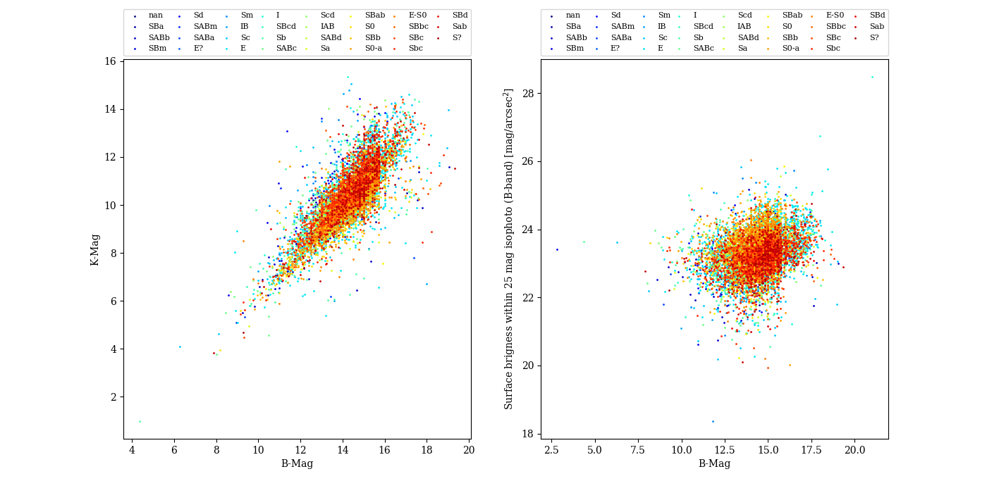
NGC.csv のプロットの例
コードの例
import pandas as pd
df = pd.read_table('NGC.csv', header=0,delimiter=";")
import matplotlib.mlab as mlab
import matplotlib.pyplot as plt
import matplotlib.cm as cm
plt.rcParams['font.family'] = 'serif'
import matplotlib.colors as colors
fig = plt.figure(figsize=(14,7.))
ax = fig.add_subplot(1, 2, 1)
num=len(set(df["Hubble"]))
usercmap = plt.get_cmap('jet')
cNorm = colors.Normalize(vmin=0, vmax=num)
scalarMap = cm.ScalarMappable(norm=cNorm, cmap=usercmap)
for i, sp in enumerate(set(df["Hubble"])):
c = scalarMap.to_rgba(i)
df_species = df[df['Hubble'] == sp]
ax.scatter(data=df_species, x='B-Mag', y='K-Mag', label=sp, color=c, s=1)
plt.xlabel("B-Mag")
plt.ylabel("K-Mag")
plt.legend(bbox_to_anchor=(0., 1.01, 1., 0.01), loc='lower left',ncol=8, mode="expand", borderaxespad=0.,fontsize=8)
ax = fig.add_subplot(1, 2, 2)
for i, sp in enumerate(set(df["Hubble"])):
c = scalarMap.to_rgba(i)
df_species = df[df['Hubble'] == sp]
ax.scatter(data=df_species, x='B-Mag', y='SurfBr', label=sp, color=c, s=1)
plt.xlabel("B-Mag")
plt.ylabel(r"Surface brigness within 25 mag isophoto (B-band) [mag/arcsec$^2$]")
plt.legend(bbox_to_anchor=(0., 1.01, 1., 0.01), loc='lower left',ncol=8, mode="expand", borderaxespad=0.,fontsize=8)
plt.savefig("ngc_bk_bs.png")
plt.show()
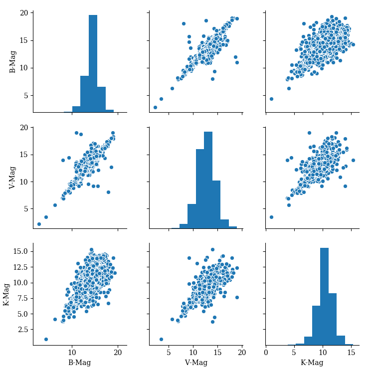
import seaborn as sns
sns.pairplot(df[df["Type"]=="G"],vars=["B-Mag","V-Mag","K-Mag"])
plt.savefig("ngc_bvk_galaxy.png")
matplotlib の scatter plot の図
seaborn の sns.pairplot の図
データベースの説明
https://github.com/mattiaverga/OpenNGC/blob/master/NGC_guide.txt に説明がある。
-
Name: Object name composed by catalog + number
NGC: New General Catalogue
IC: Index Catalogue -
Type: Object type
*: Star
**: Double star
*Ass: Association of stars
OCl: Open Cluster
GCl: Globular Cluster
Cl+N: Star cluster + Nebula
G: Galaxy
GPair: Galaxy Pair
GTrpl: Galaxy Triplet
GGroup: Group of galaxies
PN: Planetary Nebula
HII: HII Ionized region
DrkN: Dark Nebula
EmN: Emission Nebula
Neb: Nebula
RfN: Reflection Nebula
SNR: Supernova remnant
Nova: Nova star
NonEx: Nonexistent object
Dup: Duplicated object (see NGC or IC columns to find the master object)
Other: Other classification (see object notes) -
RA: Right Ascension in J2000 Epoch (HH:MM:SS.SS)
-
Dec: Declination in J2000 Epoch (+/-DD:MM:SS.SS)
-
Const: Constellation where the object is located
-
MajAx: Major axis, expressed in arcmin
-
MinAx: Minor axis, expressed in arcmin
-
PosAng: Major axis position angle (North Eastwards)
-
B-Mag: Apparent total magnitude in B filter
-
V-Mag: Apparent total magnitude in V filter
-
J-Mag: Apparent total magnitude in J filter
-
H-Mag: Apparent total magnitude in H filter
-
K-Mag: Apparent total magnitude in K filter
-
SurfBr (only Galaxies): Mean surface brigthness within 25 mag isophot (B-band), expressed in mag/arcsec2
-
Hubble (only Galaxies): Morphological type (for galaxies)
-
Cstar U-Mag (only Planetary Nebulae): Apparent magnitude of central star in U filter
-
Cstar B-Mag (only Planetary Nebulae): Apparent magnitude of central star in B filter
-
Cstar V-Mag (only Planetary Nebulae): Apparent magnitude of central star in V filter
-
M: cross reference Messier number
-
NGC: other NGC identification, if the object is listed twice in the catalog
-
IC: cross reference IC number, if the object is also listed with that identification
-
Cstar Names (only Planetary Nebulae): central star identifications
-
Identifiers: cross reference with other catalogs
-
Common names: Common names of the object if any
-
NED Notes: notes about object exported from NED
-
OpenNGC Notes: notes about the object data from OpenNGC catalog
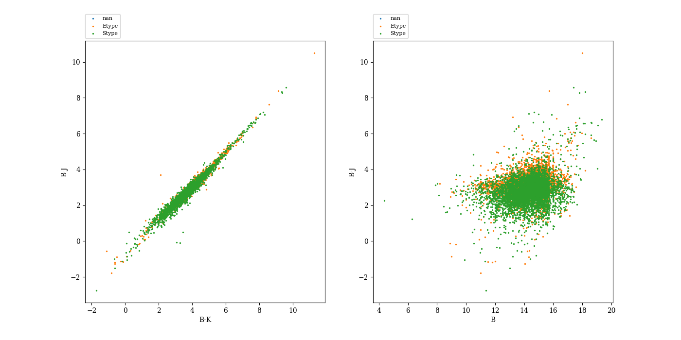
ハッブルタイプを簡略化し、Nanを除去してからプロットする方法
例えば、ハッブルタイプは数が多いので、それを簡略化したい場合もあるであろう。
その場合は、
set(df["Hubble"])
として、ハッブルタイプの種類を調べる。それを変換する辞書を作成し、変換した結果を記録する新しいコラムを作成する。
htype={'E':"Etype", 'E-S0':"Etype",  'E?':"Etype",  'I':"Etype",  'IAB':"Etype",  'IB':"Etype",  \
'S0':"Etype", 'S0-a':"Etype",  'S?':"Etype",  'SABa':"Stype",   'SABb':"Stype",  'SABc':"Stype",  'SABd':"Stype",  'SABm':"Stype",  'SBa':"Stype", \
'SBab':"Stype", 'SBb':"Stype", 'SBbc':"Stype", 'SBc':"Stype", 'SBcd':"Stype", 'SBd':"Stype", 'SBm':"Stype", 'Sa':"Stype", 'Sab':"Stype", 'Sb':"Stype",  \
'Sbc':"Stype", 'Sc':"Stype", 'Scd':"Stype", 'Sd':"Stype", 'Sm':"Stype", "nan":"Nan"}
df["htype"] = df["Hubble"]
df = df.replace({"htype":htype})
ここでは、例のため、単純にEtypeとStypeとNanの3分割する例を示した。EをEに変換すると再帰的になるのでおかしくなることはあるので、同じ文字に変換するのは避けよう。
Nanの削除方法
データの中にNanがあると困るので、必要なコラムだけを抽出し、それに対して、dropnaを実行して、Nanを削除する。
    ds = df_species.loc[:,["B-Mag","K-Mag","J-Mag"]]
    ds = ds.dropna(how='any')
サンプルコード
import pandas as pd
df = pd.read_table('NGC.csv', header=0,delimiter=";")

htype={'E':"Etype", 'E-S0':"Etype",  'E?':"Etype",  'I':"Etype",  'IAB':"Etype",  'IB':"Etype",  \
'S0':"Etype", 'S0-a':"Etype",  'S?':"Etype",  'SABa':"Stype",   'SABb':"Stype",  'SABc':"Stype",  'SABd':"Stype",  'SABm':"Stype",  'SBa':"Stype", \
'SBab':"Stype", 'SBb':"Stype", 'SBbc':"Stype", 'SBc':"Stype", 'SBcd':"Stype", 'SBd':"Stype", 'SBm':"Stype", 'Sa':"Stype", 'Sab':"Stype", 'Sb':"Stype",  \
'Sbc':"Stype", 'Sc':"Stype", 'Scd':"Stype", 'Sd':"Stype", 'Sm':"Stype", "nan":"Nan"}

df["htype"] = df["Hubble"]
df = df.replace({"htype":htype})

import matplotlib.mlab as mlab
import matplotlib.pyplot as plt
import matplotlib.cm as cm
plt.rcParams['font.family'] = 'serif'
import matplotlib.colors as colors

fig = plt.figure(figsize=(14,7.))

ax = fig.add_subplot(1, 2, 1)
for i, sp in enumerate(set(df["htype"])):
    df_species = df[df['htype'] == sp]
    ds = df_species.loc[:,["B-Mag","K-Mag","J-Mag"]]
    ds = ds.dropna(how='any')
    bk = ds["B-Mag"] - ds["K-Mag"]
    bj = ds["B-Mag"] - ds["J-Mag"]
    ax.scatter(bk,bj,label=sp, s=2)
plt.xlabel("B-K")
plt.ylabel("B-J")
plt.legend(bbox_to_anchor=(0., 1.01, 1., 0.01), loc='lower left',borderaxespad=0.,fontsize=8)

ax = fig.add_subplot(1, 2, 2)
for i, sp in enumerate(set(df["htype"])):
    df_species = df[df['htype'] == sp]
    ds = df_species.loc[:,["B-Mag","K-Mag","J-Mag"]]
    ds = ds.dropna(how='any')
    bj = ds["B-Mag"] - ds["J-Mag"]
    ax.scatter(ds["B-Mag"],bj,label=sp, s=2)
plt.xlabel("B")
plt.ylabel("B-J")
plt.legend(bbox_to_anchor=(0., 1.01, 1., 0.01), loc='lower left',borderaxespad=0.,fontsize=8)

plt.savefig("ngc_bk_bj.png")
plt.show()
生成される図