宇宙背景X線放射(CXB)をフラックス範囲を指定してpythonで計算する方法

背景

宇宙背景X線放射(CXB)を推定する場合に、トータルの明るさはいくつかを知りたいだけではなくて、撮像観測した場合は、撮像により検出された明るい点源は除いた場合に、どのくらいが空間分解せずに残っているか？を推定する必要がある。

ここでは、https://iopscience.iop.org/article/10.1086/374335 に従って、soft (1-2 keV) と hard (2-10 keV) のそれぞれをpythonで計算する方法を紹介する。

ソースコード

コードを読めばわかる人は、calc_cxbのColab を参照ください。

#!/bin/evn python 

import matplotlib.pyplot as plt
import numpy as np

# THE RESOLVED FRACTION OF THE COSMIC X-RAY BACKGROUND A. Moretti, 
# The Astrophysical Journal, Volume 588, Number 2 (2003)
# https://iopscience.iop.org/article/10.1086/374335

smax = 1e-1 # maxinum of flux range (erg cm^-2 c^-1)
smin = 1e-17 # minimum of flux range (erg cm^-2 c^-1)
n = int(1e5) # number of grid in flux 
fcut = 5e-14 # user-specified maxinum flux (erg cm^-2 c^-1)

def calc_cxb(s,fcut=5e-14, ftotal_walker=2.18e-11, plot=True, soft=True):

	if soft: # 1-2 keV
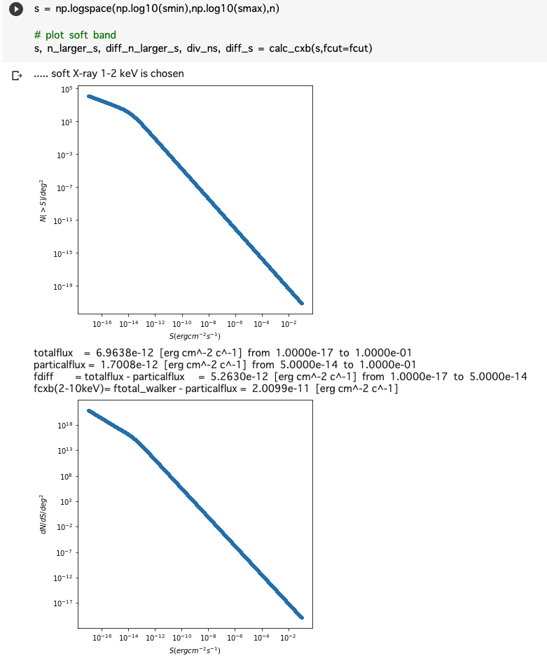
		print("..... soft X-ray 1-2 keV is chosen")
		a1=1.82; a2=0.6; s0=1.48e-14; ns=6150
		foutname="soft"
	else: # hard 2-10 keV 
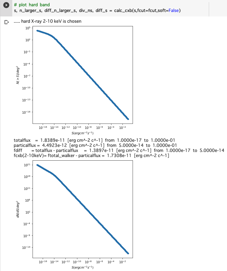
		print("..... hard X-ray 2-10 keV is chosen")
		a1=1.57; a2=0.44; s0=4.5e-15; ns=5300
		foutname="hard"


	n_larger_s = ns * 2.0e-15 ** a1 / (s**a1 + s0**(a1-a2)*s**a2) # Moretti et al. 2013, eq(2)

	if plot:
		F = plt.figure(figsize=(6,6))
		ax = plt.subplot(1,1,1)
		plt.plot(s, n_larger_s, ".", label="test")
		plt.xscale('log')
		plt.ylabel(r"$N(>S)/deg^2$")
		plt.xlabel(r"$S (erg cm^{-2} s^{-1})$")
		plt.yscale('log')
		plt.savefig(foutname + "_ns.png")
		plt.show()

	diff_n_larger_s = np.abs(np.diff(n_larger_s))
	diff_s = np.diff(s)
	div_ns = np.abs(diff_n_larger_s/diff_s)

	s_lastcut = s[:-1]
	totalflux = np.sum(div_ns*s_lastcut*diff_s) # Moretti et al. 2013, eq(4)

	fluxcut = np.where(s > fcut)[0][:-1]
	particalflux = np.sum(div_ns[fluxcut]*s_lastcut[fluxcut]*diff_s[fluxcut])
	fdiff = totalflux - particalflux 
	fcxb = ftotal_walker - particalflux # Walker et al. 2016, eq(1)

	print("totalflux    = ", "%.4e"%totalflux, " [erg cm^-2 c^-1]", " from ", "%.4e"%smin, " to ",  "%.4e"%smax)
	print("particalflux = ", "%.4e"%particalflux, " [erg cm^-2 c^-1]", " from ", "%.4e"%fcut, " to ",  "%.4e"%smax)
	print("fdiff        = totalflux - particalflux     = ", "%.4e"%fdiff, " [erg cm^-2 c^-1]", " from ", "%.4e"%smin, " to ",  "%.4e"%fcut)	
	print("fcxb(2-10keV)= ftotal_walker - particalflux = ", "%.4e"%fcxb, " [erg cm^-2 c^-1]")

	if plot:
		F = plt.figure(figsize=(6,6))
		ax = plt.subplot(1,1,1)
		plt.plot(s[:-1], div_ns, ".", label="test")
		plt.xscale('log')
		plt.ylabel(r"$dN/dS/deg^2$")
		plt.xlabel(r"$S (erg cm^{-2} s^{-1})$")
		plt.yscale('log')
		plt.savefig(foutname + "_nsdiff.png")		
		plt.show()

	return s, n_larger_s, diff_n_larger_s, div_ns, diff_s

#s = np.linspace(sexcl,smax,n)
s = np.logspace(np.log10(smin),np.log10(smax),n)

# plot soft band
s, n_larger_s, diff_n_larger_s, div_ns, diff_s = calc_cxb(s,fcut=fcut)
# plot hard band
s, n_larger_s, diff_n_larger_s, div_ns, diff_s = calc_cxb(s,fcut=fcut,soft=False)

実行結果

1-2 keV

2-10 keV

計算方法

さすがにリニアだとメモリが足りずに計算できないので、s(erg cm^-2 s^-1)空間のログで、積分はただの長方形近似を用いた。

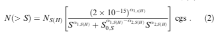
この関数は、n_larger_s = ns * 2.0e-15 ** a1 / (sa1 + s0(a1-a2)*s**a2) で計算している。

この積分は、totalflux = np.sum(div_nss_lastcutdiff_s) で計算している。

fcxb = ftotal_walker - particalflux # Walker et al. 2016, eq(1) の部分はおまけで、この論文の 2-10 keV のCXBの推定をしており、それに準じた計算を出しておいた。