ガウシアンとローレンツ関数の違い
ガウス関数はテイルが小さく、ローレンツ関数はテイルが大きい、という定性的な話だけでなく、定量的にどの程度かを確認してみよう。
ローレンツ関数の定義については,wikipedia日本語や,wikipedia英語 : Cauchy distribution がよくまとまっているので参照してください.ここでは,半値幅の整数倍で両者に定量的にどの程度の違いがでるのかを早見表的に知りたい人向けの記事になります.想定しているのは,精密分光の分野などで,複数のラインを分離したい場合で,ローレンチアンのテイル成分が無視できないか自明ではないような状況です.
ローレンツ関数の定義
平均値が0で、全積分で面積が1となるように規格化されたローレンツ関数を用いる.
\begin{align}
l(x, \gamma) &= \frac{1}{\pi \gamma ( 1 + (x/\gamma)^2)} \\
             &= \frac{l(0,\gamma)}{ 1 + (x/\gamma)^2}
\end{align}
この定義だと、x = 0 の値はガンマに依存することに注意する。定義によっては、$l(0, \gamma)$ のNormalizatioを別の変数に丸め込むこともある。
この定義では、
- $\gamma$は half-width at half-maximum (HWHM)である。
- $2\gamma$が full width at half maximum (FWHM) である。
- $2\gamma$は四分位範囲(interquartile range)である。
となる。四分位範囲はデータを大きい順番に並べ四分割(各25%)し、上位25%の点(第1四分位)と75%の点(第3四分位)の範囲を四分位範囲とする。第1四分位が正のガンマで、第3四分位が負のガンマとなる。
ガウス関数の定義
平均値が0で、全積分で面積が1となるように規格化されたガウス関数, 別名 Normal distributionを用いる。
\begin{align}
g(x, \sigma) &= \frac{1}{\sqrt{2 \pi \sigma^2}} exp( - (x/\sigma)^2/2) \\
             &= g(0, \sigma) exp( - (x/\sigma)^2/2) \\
\end{align}
この半値幅との関係は、FWHM = 2$\sigma \sqrt{2 ln2} \sim 2.35 \sigma$ である。
プロット方法
ガウシアンもローレンチアンも平均値は0として、FWHMをどちらも4とする。
# !/usr/bin/env python

import math
import matplotlib.pyplot as plt
import numpy as np

pi=math.pi

def l(x,gamma):
    return 1/(pi * gamma * ( 1 + math.pow(x/gamma,2))) # gamma = 0.5 * FWHM

def g(x,sigma):
    return math.exp(-math.pow(x/sigma,2)/2) / math.sqrt(2*pi*sigma*sigma)

fwhm = 4
hwhm = 0.5 * fwhm
gamma= 0.5 * fwhm
sigma=fwhm / 2.35 # sigma ==> FWHM

x = np.linspace(0, 10, 100)
yl = [ l(onex,gamma)/l(0,gamma) for onex in x]
yg = [ g(onex,sigma)/g(0,sigma) for onex in x]

n = np.arange(6)
iyl = [ l(hwhm*onen,gamma)/l(0,gamma) for onen in n]
iyg = [ g(hwhm*onen,sigma)/g(0,sigma) for onen in n]

plt.errorbar(x,yl, fmt="r--",label="Lorentzian FWHM = " + str(fwhm))
plt.errorbar(x,yg, fmt="b--",label="Gaussian FWHM = " + str(fwhm))

plt.errorbar(n*hwhm,iyl, fmt="ro", label="Lorentzian n x HWHM")
plt.errorbar(n*hwhm,iyg, fmt="bo", label="Gaussian n x HWHM")

plt.yscale('linear')
plt.grid(linestyle='dotted',alpha=0.5)
plt.legend(bbox_to_anchor=(-0.1, 1.0, 1.2, 0.01), loc='lower left',ncol=2, borderaxespad=0.,fontsize=8)
plt.show()

for onen,onel,oneg in zip(n,iyl,iyg):
	print(onen,onel,oneg)
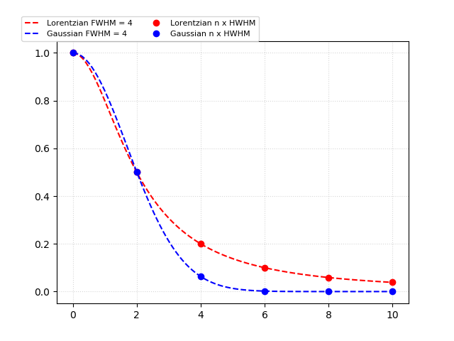
単純に両者をラインでプロットするのに加えて、FWHM(半値全幅(FWHM - Full Width at Half Maximum) ではなくて半値半幅(HWHM, Half Width at Half Maximum)の整数倍の値を重ねて点でプロットした。
N x 半値半幅(今の場合は2)のNに対して、ローレンチアンとガウシアンがどのような値になるかをまとめる。
| N | ローレンチアン | ガウシアン |
|---|---|---|
| 0 | 1.0 | 1.0 |
| 1 | 0.5 | 0.50141 |
| 2 | 0.2 | 0.06321 |
| 3 | 0.1 | 0.002003 |
| 4 | 0.058 | 1.596e-05 |
| 5 | 0.0384 | 3.199e-08 |
| 6 | 0.0270 | 1.611e-11 |
| 7 | 0.0199 | 2.041e-15 |
| 8 | 0.0153 | 6.499e-20 |
| 9 | 0.0121 | 5.203e-25 |
| 10 | 0.0099 | 1.047e-30 |
| 50 | 0.0004 | 0 |
| 100 | 1e-04 | 0 |
この表の読み方は、ローレンチアンは半値半幅の3倍(N=3)くらいで10%程度にしか下がってないが、ガウシアンは0.2%程度まで下がっている。半値半幅の10倍(N=10)でもローレンチアンは1%程度の残留成分があるのに対して、ガウシアンは実質ほぼゼロになる。
実用的な使い方
輝線の幅を計測する装置のエネルギー分解能がよくなると、自然幅が利くようになり、テイル成分の影響が無視できなくなる。例えば、自然幅のFWHMが4eVの場合、N=10 x 2eV = 20 eV 離れたとしても、1%程度の漏れこみが存在しうる。N=100 x 2eV = 200 eV 離れても 0.01% 程度の寄与が残るので、ローレンチアンのテイルは意外と侮れないのである。