パワースペクトルに位相ランダムを仮定して時系列データを生成する方法

パワースペクトルから時系列データを生成する方法

パワースペクトルから時系列データを生成には、位相が必要となる。その位相情報をランダムを仮定することで、時系列データの生成が可能になる。手法については、下記の文献に従って実装したものである。

• Timmer & Konig (1995; A&A) : http://adsabs.harvard.edu/abs/1995A%26A...300..707T

このページのスクリプトは google Colab 上で見れるように、GenRandomLightCurve_TimmerKoenight_Colab.ipynb においてます。

補足説明

P(f) はパワースペクトルのルートをとったもの(e.g., V(t)データをFFTして、V/sqrt(Hz)の単位)とします。
乱数の発生方法は、

• 実部 = (P(f) / √2) * ガウス乱数(平均=0,分散=1)
• 虚部 = (P(f) / √2) * ガウス乱数(平均=0,分散=1)

で実部と虚部を乱数で発生させ(位相をランダムに発生させることと同等)、フーリエ逆変換することで、時系列に戻す。

(補足) 実部2 + 虚部2 が「自由度の２のχ2乗分布(この平均値は2」なので、√2がでてきます。

• 実部^2+虚部^2 = P(f)^2 x (ガウス乱数^2 +ガウス乱数^2 / 2) ~ P(f)^2
• 昔の説明資料とソースコード

これに更に別のノイズを加えたい場合で、パワースペクトルがわかっている場合は、同じ長さの時系列データを生成し、足しこむことで実現できます。

対数正規分布で生成する場合はこちらを参照ください。
対数正規分布 log-normal する 1次元と2次元のデータ生成方法

スクリプトと使い方

コードをみればOKな人は、GenRandomLightCurve_TimmerKoenight_Colab.ipynb を観てください。

パラメータの設定部分で、

#debug The flag to show detailed information' default=False
#plotflag' 'The flag to plot figures' default=False
#scipyplotflag' 'The flag to plot figures of scipy' default=False    
#random_tmax', 'Max time for simulated light curve (sec)' default=100.
#random_index1', 'Index1 of simulated powerspectra ( f < cutoff )' default=-1.
#random_index2', 'Index2 of simulated powerspectra ( f >= cutoff )'default=-2.
#random_norm',   'Norm. of simulated powerspectra' default=1.0
#random_dt',     'Time resolution of simulated lightcurves (sec)' default=1.0
#random_cutoff', 'Cut off frequency of simualted powerspectra (Hz)' default=0.1
outputfilename =  "check_v1"
debug =  False
plotflag =  True
scipyplotflag =  True
random_tmax =  100
random_norm =  1.0
random_dt =    1.0
random_index1 =  -1.
random_index2 =  -2.
random_cutoff =  0.1

として、設定が変更できます。

1000秒の長さで、1秒時間ビンで、周波数のベキが -1 ( f < 0.1Hz)、 -2 ( f > 0.1Hz) のパワースペクトルで疑似的にライトカーブを生成します。出力は outputtext というディレクトリテキストが書き出されるので、それを使って解析がすぐにできる。

結果の例

上記のパラメータで計算した結果の例。

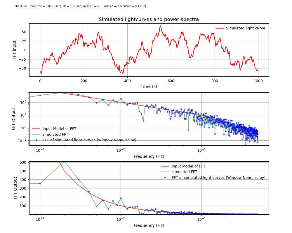
上から順に、

• 上 : 擬似的に生成されたライトカーブ
• 中 : 仮定したパワースペクトル(赤)、乱数で生成されたパワースペクトル(緑)、生成されたライトカーブをFFTしたもの(青)
• 下 : 図(中)の縦軸をログ表示

「乱数で生成されたパワースペクトル(緑)」と「生成されたライトカーブをFFTしたもの(青)」は同じになるはずで、重なることを確認するためにプロットしたものです。

その他、

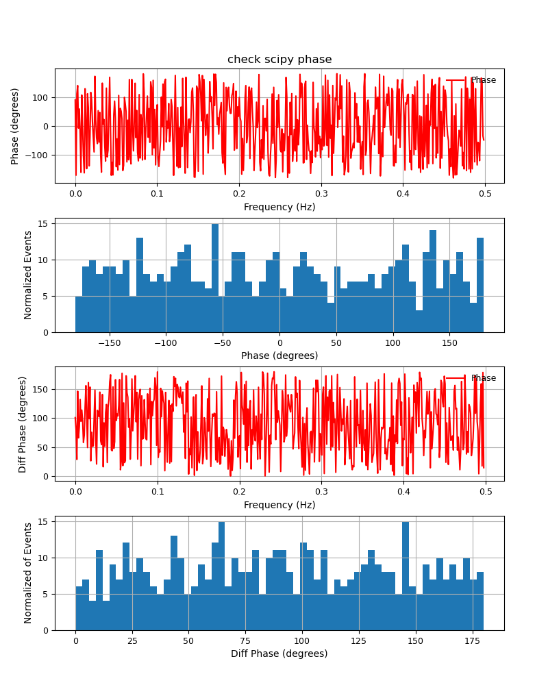
位相が本当にランダムなのかをチェックする図を生成します。

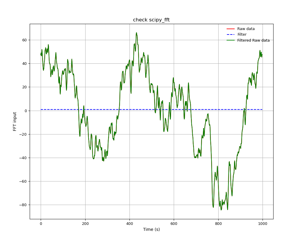
フーリエ変換する前の時系列データを確認するための図になります。ハニングや窓関数を使う場合には、時系列で窓関数のかかり具合をチェックした方がよいので、実装してあります。

ソースコード

GenRandomLightCurve_TimmerKoenight_Colab.ipynb を出しておきます。

GenRandomLightCurve_TimmerKoenight_Colab.py

#!/usr/bin/env python


""" SXS_GenRandomLC_InputRandom_simple.py is to simulated lightcurves from powerspectra baced on phases are random. 

This is a python script to check FFT.
History:
2013-08-29 ; ver 1.0; Generate Random light curves 
2013-09-27 ; ver 1.1; Delete filtering, because it bringes RMS uncertainties. 
2013-10-07 ; ver 1.2; include phase in FFT
2013-10-08 ; ver 1.3; change math.pow(s(f),2), because s(f) [RMS/sqrt(Hz)] is default. 
2015-06-28 ; ver 1.4; change math.pow(s(f),2), because s(f) [RMS/sqrt(Hz)] is default. 
2020-05-01 ; ver 1.5; updated for python3, 
2021-04-02 ; ver 1.6; renamted as GenRandomLightCurve_TimmerKoenight.py and updated for Colab

ref : https://qiita.com/yamadasuzaku/items/169d861c0a66c847a639
"""

__author__ =  'Shinya Yamada (syamada at rikkyo.ac.jp'
__version__=  '1.6'

import os
import sys
import math
import cmath
import subprocess
import numpy as np
import scipy as sp
import scipy.fftpack as sf
import matplotlib.cm as cm
import matplotlib.mlab as mlab
import matplotlib.pyplot as plt
from matplotlib.ticker import MultipleLocator, FormatStrFormatter, FixedLocator
import optparse
from matplotlib.font_manager import fontManager, FontProperties
import matplotlib.pylab as plab
import re
import sys
from numpy import linalg as LA
import csv
import random

params = {'xtick.labelsize': 9, # x ticks
          'ytick.labelsize': 9, # y ticks
          'legend.fontsize': 9
                    }

plt.rcParams.update(params)

def scipy_fft(inputarray,dt,filtname=None, pltfrag=False):

    bin = len(inputarray)
    if filtname == None:
        filt = np.ones(len(inputarray))
    elif filtname == 'hanning':
        filt = sp.hanning(len(inputarray))
    else:
        print(('No support for filtname=%s' % filtname))
        exit()

    freq = sf.fftfreq(bin,dt)[0:int(bin/2)]
    df = freq[1]-freq[0]
    fft = sf.fft(inputarray*filt,bin)[0:int(bin/2)]
    real = fft.real
    imag = fft.imag
    psd = np.abs(fft)/np.sqrt(df)/(bin/np.sqrt(2.))    
    phase = np.arctan2(np.array(real),np.array(imag)) * 180. / np.pi

    if pltfrag: 
        binarray = list(range(0,bin,1))

        # check input lightcurves
        F = plt.figure(figsize=(10,8.))
        plt.subplots_adjust(wspace = 0.1, hspace = 0.3, top=0.9, bottom = 0.08, right=0.92, left = 0.1)
        ax = plt.subplot(1,1,1)
        plt.title("check scipy_fft")
        plt.xscale('linear')
        plt.grid(True)
        plt.xlabel(r'Time (s)')
        plt.ylabel('FFT input')
        plt.errorbar(binarray, inputarray, fmt='r', label="Raw data")
        plt.errorbar(binarray, filt, fmt='b--', label="Filter")
        plt.errorbar(binarray, inputarray * filt, fmt='g', label="Filtered Raw data")
        plt.legend(numpoints=1, frameon=False, loc=1)
        outputfiguredir = "scipy_fft_check"
        subprocess.getoutput('mkdir -p ' + outputfiguredir)
        plt.savefig(outputfiguredir + "/" + "scipy_fftcheck" + "_t" + str(dt).replace(".","p") + ".png")
        plt.show()
        plt.close()

        # check phase 
        F = plt.figure(figsize=(8,10.))
        plt.subplots_adjust(wspace = 0.1, hspace = 0.3, top=0.9, bottom = 0.08, right=0.92, left = 0.1)
        ax = plt.subplot(4,1,1)
        plt.title("check scipy phase")
        plt.xscale('linear')
        plt.grid(True)
        plt.xlabel(r'Frequency (Hz)')
        plt.ylabel('Phase (degrees)')
        plt.errorbar(freq, phase, fmt='r', label="Phase")
        plt.legend(numpoints=1, frameon=False, loc=1)

        ax = plt.subplot(4,1,2)
        n, bins, patches = plt.hist(phase, bins=60, range=(-180, 180), label="Phase distribution")
        plt.xscale('linear')
        plt.grid(True)
        plt.xlabel(r'Phase (degrees)')
        plt.ylabel('Normalized Events')

        dtheta = phase[:-1] - phase[1:]
        listdtheta = []

        for dth in dtheta:
            tmpdth = dth 
            if dth > 180.:
                tmpdth = 360.0 - dth 
            elif dth < -180:
                tmpdth = 360 + dth
            elif (dth < 0. ) and dth > -180.:
                tmpdth = - dth 
            else:
                tmpdth = dth
            listdtheta.append(tmpdth)

        npdtheta = np.array(listdtheta)

        # phase diff .
        ax = plt.subplot(4,1,3)
#        plt.title("check scipy phase")
        plt.xscale('linear')
        plt.grid(True)
        plt.xlabel(r'Frequency (Hz)')
        plt.ylabel('Diff Phase (degrees)')
        plt.errorbar(freq[:-1], npdtheta, fmt='r', label="Phase")
        plt.legend(numpoints=1, frameon=False, loc=1)

        ax = plt.subplot(4,1,4)
        n, bins, patches = plt.hist(npdtheta, bins=60, range=(0, 180), label="Phase distribution")
        plt.xscale('linear')
        plt.grid(True)
        plt.xlabel(r'Diff Phase (degrees)')
        plt.ylabel('Normalized of Events')

        outputfiguredir = "scipy_fft_check"
        subprocess.getoutput('mkdir -p ' + outputfiguredir)
        plt.savefig(outputfiguredir + "/" + "scipy_fftcheck_phase" + "_t" + str(dt).replace(".","p") + ".png")
        plt.show()
        plt.close()


    return(freq, real, imag, psd, phase)


""" start main loop """

curdir = os.getcwd()

""" Setting for options """
#debug The flag to show detailed information' default=False
#plotflag' 'The flag to plot figures' default=False
#scipyplotflag' 'The flag to plot figures of scipy' default=False    
#random_tmax', 'Max time for simulated light curve (sec)' default=100.
#random_index1', 'Index1 of simulated powerspectra ( f < cutoff )' default=-1.
#random_index2', 'Index2 of simulated powerspectra ( f >= cutoff )'default=-2.
#random_norm',   'Norm. of simulated powerspectra' default=1.0
#random_dt',     'Time resolution of simulated lightcurves (sec)' default=1.0
#random_cutoff', 'Cut off frequency of simualted powerspectra (Hz)' default=0.1
outputfilename =  "check_v1"
debug =  False
plotflag =  True
scipyplotflag =  True
random_tmax =  1000
random_norm =  1.0
random_dt =    1.0
random_index1 =  -1.
random_index2 =  -2.
random_cutoff =  0.1


""" start main loop """
# Parameters    
print("\n============== input parameters ====================")
print("---- Max Time              = " + str(random_tmax) + " (s) ")
print("---- Time resolution       = " + str(random_dt) + " (s) ")
print("---- Index1 of input FFT   = " + str(random_index1)) 
print("---- Index2 of input FFT   = " + str(random_index2)) 
print("---- Cutoff frequency      = " + str(random_cutoff) + " (Hz) ")
print("---- Norm of input FFT     = " + str(random_norm)) 
print("---- Flag plotting         = " + str(plotflag))             
print("---- Flag plotting (scipy) = " + str(scipyplotflag))                 
print("---- Output Filename       = " + str(outputfilename))       
outfname = outputfilename + "_t" + "max" + str(random_tmax).replace(".","p") + "_dt"+ str(random_dt).replace(".","p") \
                          + "_index1" + str(random_index1).replace(".","p") \
                          + "_index2" + str(random_index2).replace(".","p") \
                          + "_cutoff" + str(random_cutoff).replace(".","p") \

outfnamefig = outputfilename + " " + " maxtime = " + str(random_tmax) + " (sec)  dt = "+ str(random_dt) + " (sec)"\
                          + " index1 = " + str(random_index1) \
                          + " index2 =" + str(random_index2) \
                          + " cutoff = " + str(random_cutoff) + " (Hz)"


print("---- outfname = " + str(outfname))       

print("==========================================================\n")

print("\n============== settting simulation parameters ====================")
# make time series 
random_nptime = np.arange(0,random_tmax,random_dt)
if str(len(random_nptime)%2) == '0':
    print("..... length of array is even : " + str(len(random_nptime)))
    random_nptime = random_nptime[0:-1]
    print("..... length of random_nptime must be odd, so the array is trimmed. ")

random_dlength = len(random_nptime)
print("---- Number of data length = " + str(random_dlength))
random_inputfreq = sf.fftfreq(random_dlength,random_dt)
random_df = random_inputfreq[1] - random_inputfreq[0]
print("---- Frequency resolution = " + str(random_df) + "(Hz)")
print("==========================================================\n")


print("\n" + "============== Start generating randomized powerspectra ==============")
# omit f=0, because x^-k diverge at x = 0. 
random_inputfreq_posi = random_inputfreq[1:int((random_dlength/2)+1)] # get only positive frequency

model_pow_posi = []
# input S(f) is not RMS^2/Hz but RMS/sqrt(Hz). The latter is default.
random_real_posi = []
random_imag_posi = []

for x in random_inputfreq_posi:

    tmp_pow = random_norm * np.power(x,random_index1)
    tmp_real = random_norm * np.power(x,random_index1)/np.sqrt(2) * random.gauss(0,1)
    tmp_imag = random_norm * np.power(x,random_index1)/np.sqrt(2) * random.gauss(0,1)
    if x >= random_cutoff:
        random_norm2 = random_norm * np.power(random_cutoff,random_index1) / np.power(random_cutoff,random_index2) # a x f^-k == b x f ^-l @ f = cutoff
        tmp_pow = random_norm2 * np.power(x,random_index2)
        tmp_real = random_norm2 * np.power(x,random_index2)/np.sqrt(2) * random.gauss(0,1)
        tmp_imag = random_norm2 * np.power(x,random_index2)/np.sqrt(2) * random.gauss(0,1)

    model_pow_posi.append(tmp_pow)
    random_real_posi.append(tmp_real)
    random_imag_posi.append(tmp_imag)        

#    imaghalf[-1] = 0  for Nyqist Freq and N = even. 
random_inputfft = []
random_inputfft.append( 0. ) # f = 0, no constant 
for real, imag in zip(random_real_posi, random_imag_posi):
    tmp = complex( float(real), float(imag) )
    random_inputfft.append(tmp)
for real, imag in zip(random_real_posi[-1::-1], random_imag_posi[-1::-1]):
    tmp = complex( float(real), -1. * float(imag) )
    random_inputfft.append(tmp)

random_np_inputfft = np.array(random_inputfft)
random_np_inputfft_power = np.abs(random_np_inputfft[0:int((random_dlength/2)+1)])
random_np_inputfreq = random_inputfreq[0:int((random_dlength/2)+1)]

# check input normalization from FFT intergral
random_input_rms = np.sqrt( np.sum (random_np_inputfft_power * random_np_inputfft_power) * random_df)
print("..... random_input_rms = input : RMS (f=0, white noise) = " + str(random_input_rms))

print("\n" + "============== Start Inverse FFT of Randomized Powerspectra ==============")
# IFFT is performed   
random_ifft_np_inputfft = sf.ifft(random_np_inputfft * np.sqrt(random_df) * ((random_dlength)/np.sqrt(2)))


# Define Input light curve
t = random_nptime
c = random_ifft_np_inputfft.real
print("..... check .... IFFT RMS = " + str ( np.std(c) )) 
print("..... IFFT data length = " + str(len(c)))

fNum = len(c)
Nyquist = 0.5 / random_dt
Fbin = Nyquist / (0.5 * fNum)
print("..... Nyquist (Hz) = " + str(Nyquist) + " (Hz) ")
print("..... Frequency bin size (Hz) = " + str(Fbin) + " (Hz) ")
fftnorm =  np.std(c) / (np.sqrt(Fbin) * (fNum * 0.5))
print("..... fftnorm (Random) = " + str(fftnorm))


print("\n" + "============== FFT-ing simulated Lighrcurve ==============")    
spfreq_nf,spreal_nf,spimag_nf,sppower_nf,spphase_nf = scipy_fft(c, random_dt, None, scipyplotflag)
scipy_amp_nofil = np.sqrt(2) * np.sqrt(np.sum(sppower_nf * sppower_nf) * Fbin)    
print("..... RMS from FFT(scipy, No Filter) = " + str(scipy_amp_nofil/np.sqrt(2)))


print("\n" + "============== Start plotting Lighrcurves and Powerspectra ==============")
# (1) Plot Time vs. Raw value
F = plt.figure(figsize=(10,8.))
plt.subplots_adjust(wspace = 0.1, hspace = 0.3, top=0.9, bottom = 0.08, right=0.92, left = 0.1)

plt.figtext(0.05,0.97, outfnamefig, size='x-small')


ax = plt.subplot(3,1,1)
plt.title("Simulated lightcurves and power spectra")

plt.xscale('linear')
plt.grid(True)
plt.xlabel(r'Time (s)')
plt.ylabel('FFT input')
plt.errorbar(t, c, fmt='r', label="Simulated light curve")
plt.legend(numpoints=1, frameon=False, loc='best')

# (2) Plot Freq vs. Power (log-log)
ax = plt.subplot(3,1,2)
plt.xscale('log')
plt.yscale('log')
plt.grid(True)
plt.xlabel(r'Frequency (Hz)')
plt.ylabel('FFT Output')
plt.errorbar(random_inputfreq_posi, model_pow_posi, fmt='r-', label="Input Model of FFT", alpha=0.7)
plt.errorbar(random_np_inputfreq, random_np_inputfft_power, fmt='g-', label="simulated FFT", alpha=0.5)
plt.errorbar(spfreq_nf, sppower_nf, fmt='b.', label="FFT of simulated light curves (Window None, scipy)", alpha=0.5)
plt.ylim(np.amin(sppower_nf[1:]), np.amax(sppower_nf[1:]))
plt.legend(numpoints=1, frameon=False, loc='best')


# (3) Plot Freq vs. Power (lin-lin)
ax = plt.subplot(3,1,3)
plt.xscale('log')
#    plt.xlim(0.1,0.2)
plt.yscale('linear')
plt.grid(True)
plt.xlabel(r'Frequency (Hz)')
plt.ylabel('FFT Output')

plt.errorbar(random_inputfreq_posi, model_pow_posi, fmt='r-', label="Input Model of FFT", alpha=0.7)
plt.errorbar(random_np_inputfreq, random_np_inputfft_power, fmt='g-', label="simulated FFT", alpha=0.5)
plt.errorbar(spfreq_nf, sppower_nf, fmt='b.', label="FFT of simulated light curves (Window None, scipy)", alpha=0.5)
plt.ylim(np.amin(sppower_nf[1:]), np.amax(sppower_nf[1:]))

plt.legend(numpoints=1, frameon=False, loc='best')

outputfiguredir = "outputfigure"
subprocess.getoutput('mkdir -p ' + outputfiguredir)
plt.savefig(outputfiguredir + "/" + outfname + ".png")
if plotflag:
    plt.show()
plt.close()


print("\n" + "============== dump text file ==============")
odir = "outputtext"
subprocess.getoutput('mkdir -p ' + odir)
fout = open(odir + "/" + outfname + ".txt", "w")                        
for onetime, onelc in zip(t, c):
    outstr=str(onetime) + " " + str(onelc) + "\n"
    fout.write(outstr) 
fout.close()