【学習メモ】ゼロから作るDeep Learning【5章】

ゼロから作るDeep Learning 5章

この本で重要なのは５〜７章かと思われ、
重点的に分けて記述する

誤差逆伝播法の理解の２つの方法
・「数式」による理解
・「計算グラフ（computational graph）」による理解

この本では後者について解説している

計算グラフ

計算グラフ：計算の過程をグラフによって表したもの
グラフ：データ構造としてのグラフ、複数のノードとエッジにより表現
下記図は1個１００円の林檎を購入し、消費税が10％の際の計算グラフ
順伝播：計算グラフの出発点から終着点への伝播
逆伝播：順伝播の逆の伝播

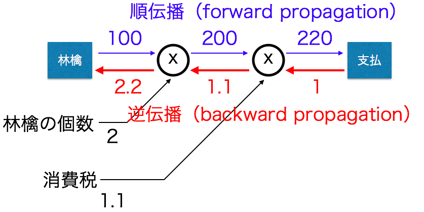
計算グラフの特徴：「局所的な計算」を伝播することによって最終的な結果を得られること
上記の図では林檎のみでしたが、他にも買い物があった際に複雑な計算になりますが
全体でどのようなことが行われていても、自分（例では林檎）に関係する情報だけから次の結果を得られます。

計算グラフのメリット：逆方向の伝播によって「微分」を効率良く計算できる

計算グラフの逆伝播

ニューラルネットワークの重みパラメータの損失関数の勾配は数値微分によって求めると計算に時間がかかる。
そのため誤差逆伝播法を行う
誤差伝播法：重みパラメータの勾配の計算を効率良く行う手法

y=f(x)という計算があるとした逆伝播

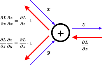
加算レイヤ

z=x+yの微分は \\
\frac{\partial z}{\partial x} = 1 \\
\frac{\partial z}{\partial y} = 1 

これを計算グラフに示すと

コードにすると

class AddLayer:
    # コンストラクタ
    def __init__(self):
        self.x = None
        self.y = None

    def forward(self, x, y):
        self.x = x
        self.y = y
        out = x+y

        return out

    def backward(self, dout):
        dx = dout * 1
        dy = dout * 1

        return dx, dy

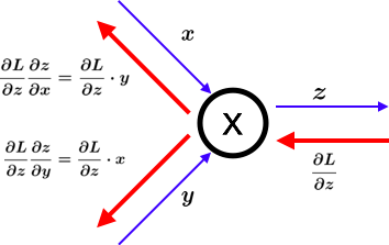
乗算レイヤ

z=x*yの微分は \\
\frac{\partial z}{\partial x} = y \\
\frac{\partial z}{\partial y} = x 

これを計算グラフに示すと

コードにすると

class MulLayer:
    # コンストラクタ
    # self = Javaのthis
    def __init__(self):
        self.x = None
        self.y = None

    def forward(self, x, y):
        self.x = x
        self.y = y
        out = x*y

        return out

    def backward(self, dout):
        dx = dout * self.y
        dy = dout * self.x


        return dx, dy

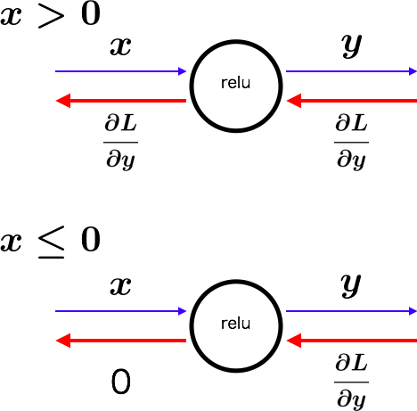
Reluレイヤ

y = \left\{
\begin{array}{ll}
x & (x \geq 0) \\
0 & (x \lt 0)
\end{array}
\right.

\frac{\partial y}{\partial x} = \left\{
\begin{array}{ll}
1 & (x \geq 0) \\
0 & (x \lt 0)
\end{array}
\right.

コードにすると

#ReLUレイヤ
class Relu:
    def __init__(self):
        self.mask = None

    def forward(self, x):
        self.mask = (x<=0)
        out = x.copy()
        out[self.mask] = 0

        return out

    def backward(self, dout):
        dout[self.mask] = 0
        dx = dout

        return dx

Sigmoidレイヤ

sigmoid関数　y=\frac{1}{1+\exp(-x)} \\

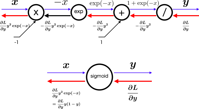
計算グラフの補足

\begin{align}

f(x)&=-x \\
\Rightarrow　f'(x)&=-1\\
f(x)&=\exp(x) \\
\Rightarrow　f'(x)&=\exp(x)\\
f(x)&=x+1 \\
\Rightarrow　f'(x)&=1\\
f(x)&=1/x \\
\Rightarrow　f'(x)&=-1/x^2=-f(x)^2\\

\end{align}

\begin{align}

\frac{\partial L}{\partial y}y^2\exp(-x) &=\frac{\partial L}{\partial y}y\frac{\exp(-x)}{1+\exp(-x)} \\
&=\frac{\partial L}{\partial y}y(1-y) \\

\end{align}

コードにすると

# Sigmoidレイヤ
class Sigmoid:
    def __init__(self):
        self.out = None

    def forward(self, x):
        out = 1 / (1 + np.exp(-x))
        self.out = out

        return out

    def backward(self, dout):
        dx = dout * (1.0 - self.out) * self.out

        return dx

Affineレイヤ

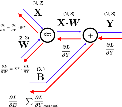
コードにすると

# バッチ版Affineレイヤ
class Affine:
    def __init__(self, W, b):
        self.W = W
        self.b = b
        self.x = None
        self.dW = None
        self.db = None

    def forward(self, x):
        self.x = x
        out = np.dot(x, self.W) + self.b

        return out

    def backward(self, dout):
        dx = np.dot(dout, self.W.T)
        self.dW = np.dot(self.x.T, dout)
        self.db = np.dot(dout, axis=0)

        return dx

証明（N＝１の単純な場合）

\begin{align}
\frac{\partial L}{\partial Y} \cdot W^T&=

\bigr(\begin{matrix}
\frac{\partial L}{\partial y_1} & 
\frac{\partial Y}{\partial y_2}& 
\frac{\partial Y}{\partial y_2}
\end{matrix}\bigr)
\Biggl(
\begin{matrix}w_{11} & w_{21} \\
w_{12} & w_{22} \\ 
w_{13} & w_{23} 
\end{matrix}\Biggr)\\

&=\bigl(\begin{matrix}
\frac{\partial L}{\partial y_1}w_{11}+
\frac{\partial L}{\partial y_2}w_{12}+
\frac{\partial L}{\partial y_3}w_{13} &
\frac{\partial L}{\partial y_1}w_{21}+
\frac{\partial L}{\partial y_2}w_{22}+
\frac{\partial L}{\partial y_3}w_{23}
\end{matrix}\bigr)\\
&=\bigl(\begin{matrix}
\frac{\partial L}{\partial y_1}\frac{\partial y_1}{\partial x_1}
+\frac{\partial L}{\partial y_2}\frac{\partial y_2}{\partial x_1}
+\frac{\partial L}{\partial y_3}\frac{\partial y_3}{\partial x_1} &
\frac{\partial L}{\partial y_1}\frac{\partial y_1}{\partial x_2}
+\frac{\partial L}{\partial y_2}\frac{\partial y_2}{\partial x_2}
+\frac{\partial L}{\partial y_3}\frac{\partial y_3}{\partial x_2}
\end{matrix}\bigr)\\
&=\bigl(
\begin{matrix}
\frac{\partial L}{\partial Y}\frac{\partial Y}{\partial x_1} &
\frac{\partial L}{\partial Y}\frac{\partial Y}{\partial x_2} 
\end{matrix}\bigr)\\
&=\frac{\partial L}{\partial X}\\


X^T \cdot \frac{\partial L}{\partial Y} 
&=\Bigl(\begin{matrix}
x_1\\
x_2
\end{matrix}\Bigr)
\cdot
\bigr(\begin{matrix}
\frac{\partial L}{\partial y_1} &
\frac{\partial L}{\partial y_2} &
\frac{\partial L}{\partial y_3}
\end{matrix}\bigr)\\
&=
\bigr(\begin{matrix}
x_1\frac{\partial L}{\partial y_1} &
x_1\frac{\partial L}{\partial y_2} &
x_1\frac{\partial L}{\partial y_3}\\
x_2\frac{\partial L}{\partial y_1} &
x_2\frac{\partial L}{\partial y_2} &
x_2\frac{\partial L}{\partial y_3}
\end{matrix}\bigr)\\
&=
\bigr(\begin{matrix}
\frac{\partial L}{\partial y_1}x_1 &
\frac{\partial L}{\partial y_2}x_1 &
\frac{\partial L}{\partial y_3}x_1\\
\frac{\partial L}{\partial y_1}x_2 &
\frac{\partial L}{\partial y_2}x_2 &
\frac{\partial L}{\partial y_3}x_2
\end{matrix}\bigr)\\
&=
\bigr(\begin{matrix}
\frac{\partial L}{\partial y_1}\frac{\partial y_1}{\partial w_{11}} &
\frac{\partial L}{\partial y_2}\frac{\partial y_2}{\partial w_{12}} &
\frac{\partial L}{\partial y_3}\frac{\partial y_3}{\partial w_{13}}\\
\frac{\partial L}{\partial y_1}\frac{\partial y_1}{\partial w_{21}} &
\frac{\partial L}{\partial y_2}\frac{\partial y_2}{\partial w_{22}} &
\frac{\partial L}{\partial y_3}\frac{\partial y_3}{\partial w_{23}}
\end{matrix}\bigr)\\
&=
\bigr(\begin{matrix}
\frac{\partial L}{\partial w_{11}} &
\frac{\partial L}{\partial w_{12}} &
\frac{\partial L}{\partial w_{13}}\\
\frac{\partial L}{\partial w_{21}} &
\frac{\partial L}{\partial w_{22}} &
\frac{\partial L}{\partial w_{23}}
\end{matrix}\bigr)\\
&=\frac{\partial L}{\partial W}\\


計算補足\\
Y&=X \cdot W+B\\
y_i&=x_1w_{1i}+x_2w_{2i}+b_i\\
例）\frac{\partial y_3}{\partial w_{23}}&=x_2

\end{align}

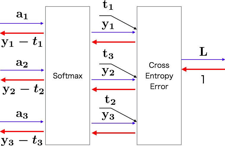
Softmax-with-Lossレイヤ

\begin{align}

&(y_1, y_2, y_3):Softmaxレイヤの出力\\
&(t_1, t_2, t_3):教師データ\\
\\
&つまり(y_1-t_1, y_2-t_2, y_3-t_3)は\\
&Softmaxレイヤの出力と教師ラベルの差\\

\end{align}

# SoftmaxWithLoss
class SofmaxWithLoss:
    def __init(self):
        self.loss = None
        self.y = None
        self.t = None

    def forward(self, x, t):
        self.t = t
        self.y = sofmax(x)
        self.loss = cross_entropy_error(self.y, self.t)

        return self.loss

    def backward(self, dout=1):
        batch_size = self.t.shape[0]
        dx - (self.y - self.t) / bath_size

        return dx

誤差逆伝播法の実装

誤差逆伝播法に対応したニューラルネットワークの実装

上記レイヤをレゴブロックのように必要なレイヤを単純に追加するだけでニューラルネットワークを作ることができる
ソースは上がっているのそのままに一部コメントを追加

# coding: utf-8
import sys, os
sys.path.append(os.pardir)  # 親ディレクトリのファイルをインポートするための設定
import numpy as np
from common.layers import *
from common.gradient import numerical_gradient
from collections import OrderedDict


class TwoLayerNet:

    #-------------------------------------------------
    # __init__:初期化を行う
    #     @self
    #     @input_size:入力層のニューロンの数
    #     @hidden_size:隠れ層のニューロンの数
    #     @output_size:出力層のニューロンの数
    #     @weight_init_std:重み初期化時のガウス分布スケール
    #-------------------------------------------------
    def __init__(self, input_size, hidden_size, output_size, weight_init_std = 0.01):


        # params:ニューラルネットのパラメータを保持する辞書型変数
        # 重みの初期化
        self.params = {}
        self.params['W1'] = weight_init_std * np.random.randn(input_size, hidden_size)
        self.params['b1'] = np.zeros(hidden_size)
        self.params['W2'] = weight_init_std * np.random.randn(hidden_size, output_size) 
        self.params['b2'] = np.zeros(output_size)

        # layer:ニューラルネットワークのレイヤを保持する「順序付き」辞書型変数
        # レイヤの生成:順序付きで保存しているのがポイント
        #           これにより順伝播ではそのまま、逆伝播では逆からレイヤを呼び出すだけでOK
        self.layers = OrderedDict()
        self.layers['Affine1'] = Affine(self.params['W1'], self.params['b1'])
        self.layers['Relu1'] = Relu()
        self.layers['Affine2'] = Affine(self.params['W2'], self.params['b2'])

        # ニューラルネットワークの最後のレイヤ:ここではSoftmaxWithLossレイヤ
        self.lastLayer = SoftmaxWithLoss()


    #-------------------------------------------------
    # predict:認識（推論）を行う
    #     @self
    #     @x:画像データ（入力データ）
    #-------------------------------------------------
    def predict(self, x):
        for layer in self.layers.values():
            x = layer.forward(x)

        return x


    #-------------------------------------------------
    # loss:損失関数を求める
    #     @self
    #     @x:画像データ（入力データ）
    #     @t:教師データ
    #-------------------------------------------------
    def loss(self, x, t):
        y = self.predict(x)
        return self.lastLayer.forward(y, t)


    #-------------------------------------------------
    # accuracy:認識精度を求める
    #     @self
    #     @x:画像データ（入力データ）
    #     @t:教師データ
    #-------------------------------------------------
    def accuracy(self, x, t):
        y = self.predict(x)
        y = np.argmax(y, axis=1)
        if t.ndim != 1 : t = np.argmax(t, axis=1)

        accuracy = np.sum(y == t) / float(x.shape[0])
        return accuracy


    #-------------------------------------------------
    # numerical_gradient:重みパラメータに対する勾配を数値微分によって求める（〜４章までと同様）
    #     @self
    #     @x:画像データ（入力データ）
    #     @t:教師データ
    #-------------------------------------------------
    def numerical_gradient(self, x, t):
        loss_W = lambda W: self.loss(x, t)

        grads = {}
        grads['W1'] = numerical_gradient(loss_W, self.params['W1'])
        grads['b1'] = numerical_gradient(loss_W, self.params['b1'])
        grads['W2'] = numerical_gradient(loss_W, self.params['W2'])
        grads['b2'] = numerical_gradient(loss_W, self.params['b2'])

        return grads


    #-------------------------------------------------
    # gradient:重みパラメータに対する勾配を誤差逆伝播法によって求める
    #     @self
    #     @x:画像データ（入力データ）
    #     @t:教師データ
    #-------------------------------------------------
    def gradient(self, x, t):

        # ポイント:実際にレイヤとして実装した伝播を動かしている

        # forward:順伝播
        self.loss(x, t)

        # backward:逆伝播
        dout = 1
        dout = self.lastLayer.backward(dout)

        layers = list(self.layers.values())
        layers.reverse()
        for layer in layers:
            dout = layer.backward(dout)

        # 設定
        grads = {}
        grads['W1'], grads['b1'] = self.layers['Affine1'].dW, self.layers['Affine1'].db
        grads['W2'], grads['b2'] = self.layers['Affine2'].dW, self.layers['Affine2'].db

        return grads

誤差逆伝播法の勾配確認

このソースは単に順伝播と逆伝播で勾配の差がほぼないことを確認するためのソース

# coding: utf-8
import sys, os
sys.path.append(os.pardir)  # 親ディレクトリのファイルをインポートするための設定
import numpy as np
from dataset.mnist import load_mnist
from two_layer_net import TwoLayerNet

# データの読み込み
(x_train, t_train), (x_test, t_test) = load_mnist(normalize=True, one_hot_label=True)

network = TwoLayerNet(input_size=784, hidden_size=50, output_size=10)

x_batch = x_train[:3]
t_batch = t_train[:3]

grad_numerical = network.numerical_gradient(x_batch, t_batch)
grad_backprop = network.gradient(x_batch, t_batch)

for key in grad_numerical.keys():
    diff = np.average( np.abs(grad_backprop[key] - grad_numerical[key]) )
    print(key + ":" + str(diff))

私の環境での実行結果
W1:2.61413510374e-13 > 2.61*0.1^-13
W2:1.04099504538e-12 > 1.04*0.1^-12
b1:9.1090807423e-13 > 9.1*0.1^-13
b2:1.20348173094e-10 > 1.2*0.1^-10

誤差逆伝播法を使った学習

このソースは要はミニバッチで繰り返し学習（重み、バイアスの更新）をしているだけ

# coding: utf-8
import sys, os
sys.path.append(os.pardir)

import numpy as np
from dataset.mnist import load_mnist
from two_layer_net import TwoLayerNet

# データの読み込み
(x_train, t_train), (x_test, t_test) = load_mnist(normalize=True, one_hot_label=True)

network = TwoLayerNet(input_size=784, hidden_size=50, output_size=10)

iters_num = 10000
train_size = x_train.shape[0]
batch_size = 100
learning_rate = 0.1

train_loss_list = []
train_acc_list = []
test_acc_list = []

iter_per_epoch = max(train_size / batch_size, 1)

for i in range(iters_num):
    batch_mask = np.random.choice(train_size, batch_size)
    x_batch = x_train[batch_mask]
    t_batch = t_train[batch_mask]

    # 勾配
    #grad = network.numerical_gradient(x_batch, t_batch)
    grad = network.gradient(x_batch, t_batch)

    # 更新
    for key in ('W1', 'b1', 'W2', 'b2'):
        network.params[key] -= learning_rate * grad[key]

    loss = network.loss(x_batch, t_batch)
    train_loss_list.append(loss)

    if i % iter_per_epoch == 0:
        train_acc = network.accuracy(x_train, t_train)
        test_acc = network.accuracy(x_test, t_test)
        train_acc_list.append(train_acc)
        test_acc_list.append(test_acc)
        print(train_acc, test_acc)