Google Colaboratory上で勾配降下法を可視化する

はじめに

以前(2018/07/31)、「Google Colaboratory上でmatplotlibのアニメーションを再生する」という記事を書きました。

下記サイトでは勾配降下法 (Gradient Descent)のグラフをアニメーション化しており、かっこいいです。
ロジスティック回帰 (勾配降下法 / 確率的勾配降下法) を可視化する
後で、勾配降下法 (Gradient Descent)のグラフをアニメーション化して公開する予定です。

記事内ではGoogle Colaboratory上でmatplotlibのアニメーションする方法の紹介に留めて、自分で組むことをしていなかったですが、ゴールデンウィークで時間が出来たのでやってみました。

アニメーション

Matplotlibアニメーションを使用しています。
ただ、Google ColaboratoryではJupyter notebook と同じ方法で表示することが出来ません。

参照:Google Colaboratory上でmatplotlibのアニメーションを再生する

matplotlib.animationパッケージ には、データを動的に可視化するためのArtistAnimation() と FuncAnimation() が用意されています。

• animation.ArtistAnimation
  事前に用意してあるデータでアニメーションを作成します。
• animation.FuncAnimation
  関数を繰り返し呼び出すことでアニメーションを作成します。

今回は、ArtistAnimation を使用しました。

# アニメーション開始
ani = animation.ArtistAnimation(fig, objs, interval=100, blit=True)

• 引数
  • fig: Figure オブジェクト
  • objs: 各フレームを構成する Artist の一覧
  • interval: 各フレームのインターバルを ms で指定する
  • bilit: blitting を使用して描画を高速化するかどうか。デフォルトは False

JavaScriptウィジェットとして埋め込む

rc('animation', html='jshtml')
ani

動画(mp4)として埋め込む

準備として、ffmpeg をインストールする必要があります。
Google Colaboratoryでは、先頭に「!」を付けて実行すればいいです。

# To make an animation, we need ffmpeg
!apt-get update && apt-get install ffmpeg

ffmpegを使用してmp4形式に出力します。

plt.rcParams['animation.ffmpeg_path'] = '/usr/bin/ffmpeg' # For google colab
HTML(ani.to_html5_video())

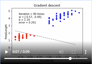
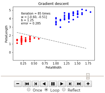
勾配降下法

今回は、irisのデータをロジスティック回帰で線形分離していくアニメーションとなる。
irisのデータは、Web上から取得しています。
参照:Google ColaboratoryでGitHubのCSVデータをpandasに読み込む

数値解析の分野では勾配降下法を最急降下法と呼びますが、勾配降下法の中にもいくつかの方法が存在します。

• 最急降下法(Gradient Descent) ※デフォルト
• 確率的勾配降下法(Stochastic Gradient Descent - SDG)
• ミニバッチ確率的勾配降下法(Minibatch SGD - MSGD)

最急降下法(Gradient Descent)

パラメーター更新の式です。

\displaystyle \theta_j := \theta_j - \eta \sum_{i=1}^n \Biggl(f_{\theta}(x)-y^{(i)}\Biggr)x_j

最急降下法は学習データのすべての誤差の合計を取ってからパラメーターを更新します。学習データが多いと計算コストがとても大きくなってしまいます。また、学習データが増えるたびに全ての学習データで再学習が必要となってしまいます。

最急降下法

import numpy as np
import pandas as pd
import urllib.request
from io import StringIO

import matplotlib.pyplot as plt
from matplotlib import animation, rc
from IPython.display import HTML

url = "https://raw.githubusercontent.com/pandas-dev/pandas/master/pandas/tests/data/iris.csv"

#csvを読み込む関数
res = urllib.request.urlopen(url)
res = res.read().decode("utf-8")
iris = pd.read_csv(StringIO(res))

np.random.seed(1)
# 描画領域のサイズ
FIGSIZE = (5, 3.5)

# 2 クラスにするため、setosa, versicolor のデータのみ抽出
data = iris[:100]

# 説明変数は 2つ = 2 次元
columns = ['PetalWidth', 'PetalLength']

x = data[columns]     # データ (説明変数)
y = data['Name']      # ラベル (目的変数)

y = (y == 'Iris-setosa').astype(int)

ani = None

def p_y_given_x(x, w, b):
    # x, w, b から y の予測値 (yhat) を計算
    def sigmoid(a):
        return 1.0 / (1.0 + np.exp(-a))
    return sigmoid(np.dot(x, w) + b)

def grad(x, y, w, b):
    # 現予測値から勾配を計算
    error = y - p_y_given_x(x, w, b)
    w_grad = -np.mean(x.T * error, axis=1)
    b_grad = -np.mean(error)
    return w_grad, b_grad

def gd(x, y, w, b, eta=0.1, num=100):
    for i in range(1, num):
        # 入力をまとめて処理
        w_grad, b_grad = grad(x, y, w, b)
        w -= eta * w_grad
        b -= eta * b_grad
        e = np.mean(np.abs(y - p_y_given_x(x, w, b)))
        yield i, w, b, e

def plot_x_by_y(x, y, colors, ax=None):
    if ax is None:
        # 描画領域を作成
        fig = plt.figure(figsize=FIGSIZE)

        # 描画領域に Axes を追加、マージン調整
        ax = fig.add_subplot(1, 1, 1)
        fig.subplots_adjust(bottom=0.15)

    x1 = x.columns[0]
    x2 = x.columns[1]
    for (species, group), c in zip(x.groupby(y), colors):
        ax = group.plot(kind='scatter', x=x1, y=x2,
                        color=c, ax=ax, figsize=FIGSIZE)
    return ax

def plot_logreg(x, y, fitter, fig, title):
    # 描画領域に Axes を追加、マージン調整
    ax = fig.add_subplot(1, 1, 1)
    fig.subplots_adjust(bottom=0.15)
    # データ, 表題を描画
    ax = plot_x_by_y(x, y, colors=['blue', 'red'], ax=ax)
    ax.set_title(title)

    # 回帰直線描画用の x 座標
    bx = np.arange(x.iloc[:, 0].min(), x.iloc[:, 0].max(), 0.1)

    # w, b の初期値を作成
    w, b = np.zeros(2), 0
    # 勾配法の関数からジェネレータを生成
    gen = fitter(x, y, w, b)
    # ジェネレータを実行し、勾配法 1ステップごとの結果を得る
    for i, w, b, e in gen:
        # 回帰直線の y 座標を計算
        by = -b/w[1] - w[0]/w[1]*bx
        # 回帰直線を生成
        l = ax.plot(bx, by, color='gray', linestyle='dashed')
        # 描画するテキストを生成
        wt = """Iteration = {0} times
w = [{1[0]:.2f}, {1[1]:.2f}]
b = {2:.2f}
error = {3:.3}""".format(i, w, b, e)
        # axes 上の相対座標 (0.1, 0.9) に text の上部を合わせて描画
        t = ax.text(0.1, 0.9, wt, va='top', transform=ax.transAxes)
        # 描画した line, text をアニメーション用の配列に入れる
        objs.append(tuple(l) + (t, ))


# 勾配降下法 (Gradient Descent)
# 描画領域を作成
fig = plt.figure(figsize=FIGSIZE)
# 描画オブジェクト保存用
objs = []
plot_logreg(x, y, gd, fig, 'Gradient descent')

# アニメーション開始
ani = animation.ArtistAnimation(fig, objs, interval=100, blit=True)

# 動画表示(mp4)
plt.rcParams['animation.ffmpeg_path'] = '/usr/bin/ffmpeg' # For google colab
HTML(ani.to_html5_video())

# JavaScriptウィジェット
#rc('animation', html='jshtml')
#ani

※動画はmp4からgifに手動変換しています。

確率的勾配降下法(Stochastic Gradient Descent / SGD)

\theta_j := \theta_j - \eta \Biggl(f_{\theta} (x) - y^{(k)}\Biggr){x_j}

※式中の$k$ は、パラメーター更新毎にランダムに選ばれたインデックス

大きな違いとして、確率的勾配降下法ではシグマ$\sum$ (1～nまで合計)が取れています。

その分、計算コストは少なくなる。

確率的勾配降下法は学習データをシャッフルした上で学習データの中からランダムに1つを取り出して誤差を計算し、パラメーターを更新をします。勾配降下法ほどの精度は無いが増えた分だけの学習データのみで再学習する(重みベクトルの初期値は前回の学習結果を流用)ため再学習の計算量が圧倒的に低くなります。

確率的勾配降下法

# 確率的勾配降下法 (Stochastic Gradient Descent / SGD)
def sgd(x, y, w, b, eta=0.1, num=4):
    for i in range(1, num):
        for index in range(x.shape[0]):
            # 一行ずつ処理
            _x = x.iloc[[index], ]
            _y = y.iloc[[index], ]
            w_grad, b_grad = grad(_x, _y, w, b)
            w -= eta * w_grad
            b -= eta * b_grad
            e = np.mean(np.abs(y - p_y_given_x(x, w, b)))
            yield i, w, b, e

# index と同じ長さの配列を作成し、ランダムにシャッフル
indexer = np.arange(x.shape[0])
np.random.shuffle(indexer)

# x, y を シャッフルされた index の順序に並び替え
x = x.iloc[indexer, ]
y = y.iloc[indexer, ]

# 描画領域を作成
fig = plt.figure(figsize=FIGSIZE)
# 描画オブジェクト保存用
objs = []
plot_logreg(x, y, sgd, fig, 'Stochastic gradient descent')
# アニメーション開始
ani = animation.ArtistAnimation(fig, objs, interval=100, blit=True)

# 動画表示(mp4)
plt.rcParams['animation.ffmpeg_path'] = '/usr/bin/ffmpeg' # For google colab
HTML(ani.to_html5_video())

# JavaScriptウィジェット
#rc('animation', html='jshtml')
#ani

※動画はmp4からgifに手動変換しています。

ミニバッチ確率的勾配降下法(Minibatch SGD / MSGD)

\displaystyle \theta_j := \theta_j - \eta \sum_{k\in K} \Biggl(f_{\theta}(x) - y^{(k)}\Biggr)x_j

ここでシグマが付くのですが、これはインデックスの集合となります。

たとえば学習データが100個あると考えた時に、$m=10$ だったら、$K={61,53,59,16,30,21,85,31,51,10}$ みたいにランダムに10個のインデックスの集合を作って、パラメーターの更新を繰り返すことになります。

ミニバッチ確率的勾配降下法は最急降下法と確率的勾配降下法の間を取ったような形となります。 最急降下法では時間がかかりすぎ、確率的勾配降下法では一つ一つのデータにかなり揺さぶられることになるので、学習データの中からランダムにいくつかのデータを取り出して誤差を計算、パラメーターを更新をします。このときの一回に取り出すデータの数をバッチサイズと呼びます。

ミニバッチ確率的勾配降下法

# ミニバッチ確率的勾配降下法 (Minibatch SGD / MSGD)
def msgd(x, y, w, b, eta=0.1, num=25, batch_size=10):
    for i in range(1, num):
        for index in range(0, x.shape[0], batch_size):
            # index 番目のバッチを切り出して処理
            _x = x[index:index + batch_size]
            _y = y[index:index + batch_size]
            w_grad, b_grad = grad(_x, _y, w, b)
            w -= eta * w_grad
            b -= eta * b_grad
            e = np.mean(np.abs(y - p_y_given_x(x, w, b)))
            yield i, w, b, e

# index と同じ長さの配列を作成し、ランダムにシャッフル
indexer = np.arange(x.shape[0])
np.random.shuffle(indexer)

# x, y を シャッフルされた index の順序に並び替え
x = x.iloc[indexer, ]
y = y.iloc[indexer, ]

# 描画領域を作成
fig = plt.figure(figsize=FIGSIZE)
# 描画オブジェクト保存用
objs = []
plot_logreg(x, y, msgd, fig, 'Minibatch SGD')
# アニメーション開始
ani = animation.ArtistAnimation(fig, objs, interval=100, blit=True)

# 動画表示(mp4)
plt.rcParams['animation.ffmpeg_path'] = '/usr/bin/ffmpeg' # For google colab
HTML(ani.to_html5_video())

# JavaScriptウィジェット
#rc('animation', html='jshtml')
#ani

※動画はmp4からgifに手動変換しています。

最後に

こうして可視化して見比べてみると違いが分かっていいですね。