[Python3]MT5からデータを取得してcloseと200EMAとボリバンを描画する

まえがき

Python3とMT5を連携させて自動売買システムを作りたいと思ったので、完成までにかかる工数を概算するために少し手を動かしました。
とりあえず動くようにした状態なので、コードは全く整理されていません。
今後完成させるかどうかは未定ですが、現時点の汚いコードでも誰かの役に立つかもと思い記事にしました。

環境

• Visual Studio Code Version: 1.57.0
• Python3.8.6
• numpy: 1.20.3
• pandas: 1.1.3
• TA-Lib: 0.4.20
• pip: 21.1.2
• MetaTrader5: 5.0.33
• matplotlib: 3.3.2

描画結果

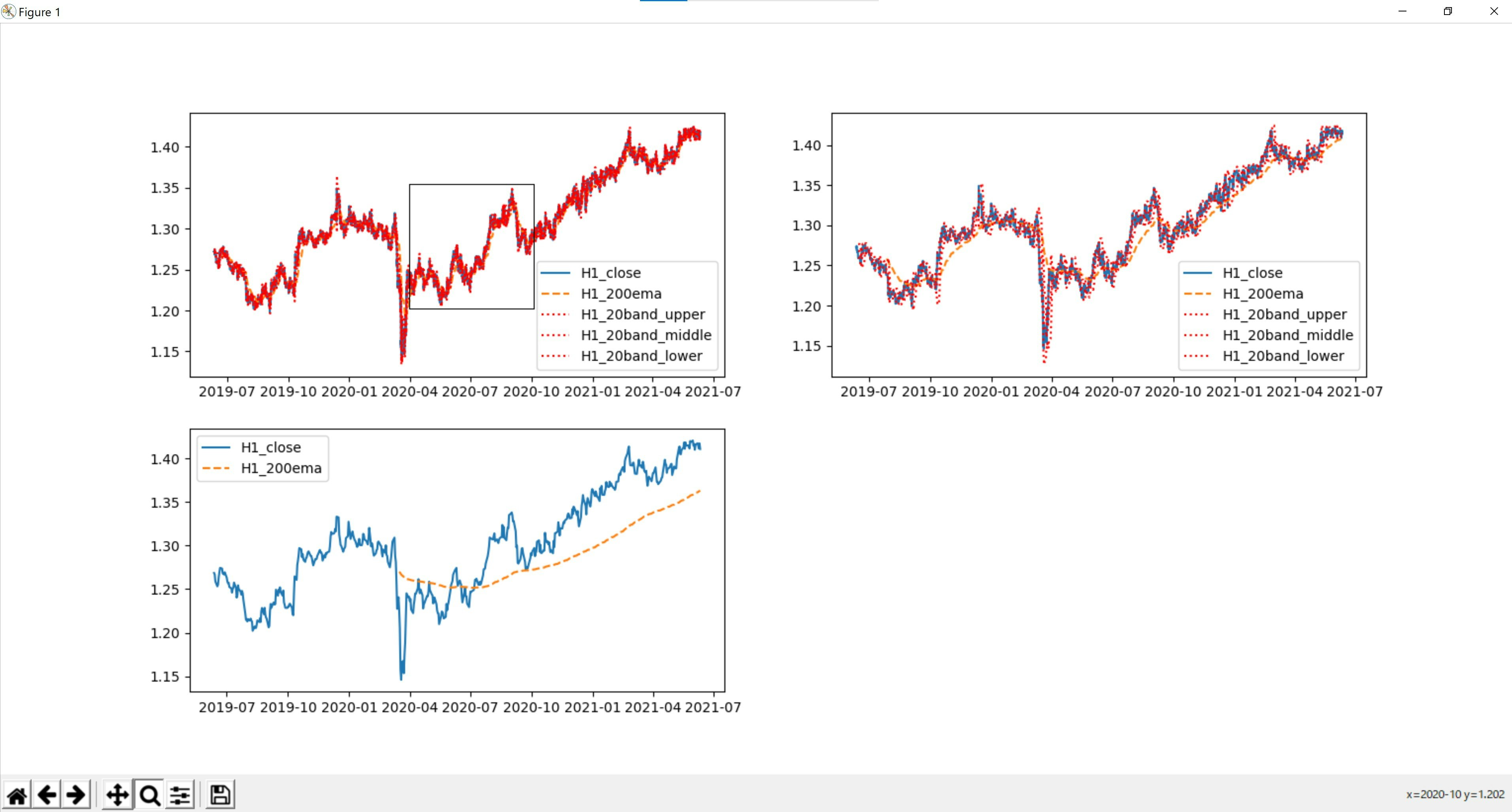
図1: 描画直後

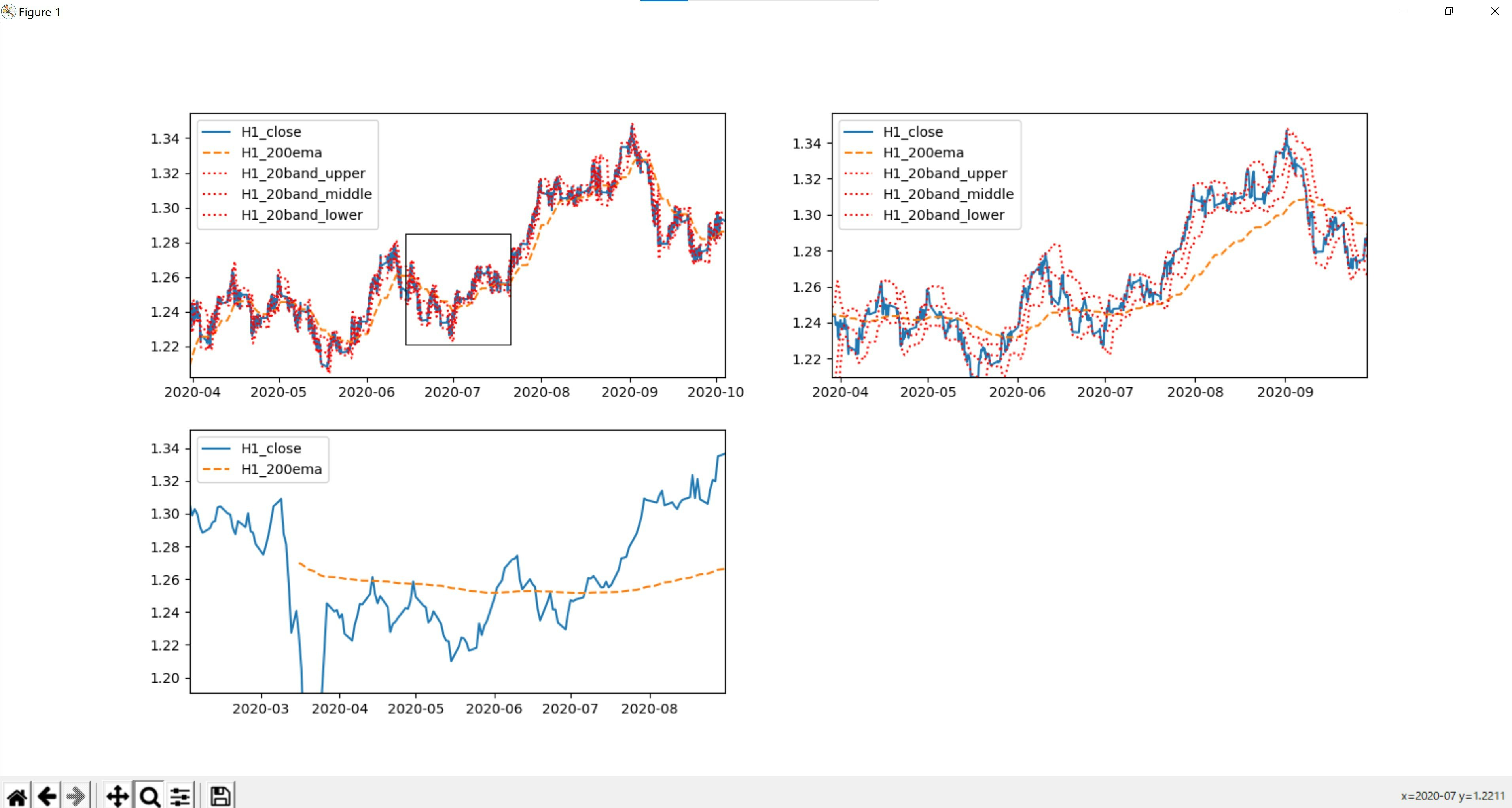
図2: 図1の左上の図の矩形選択部分を拡大。他2つの図に関しても同様の部分を拡大。

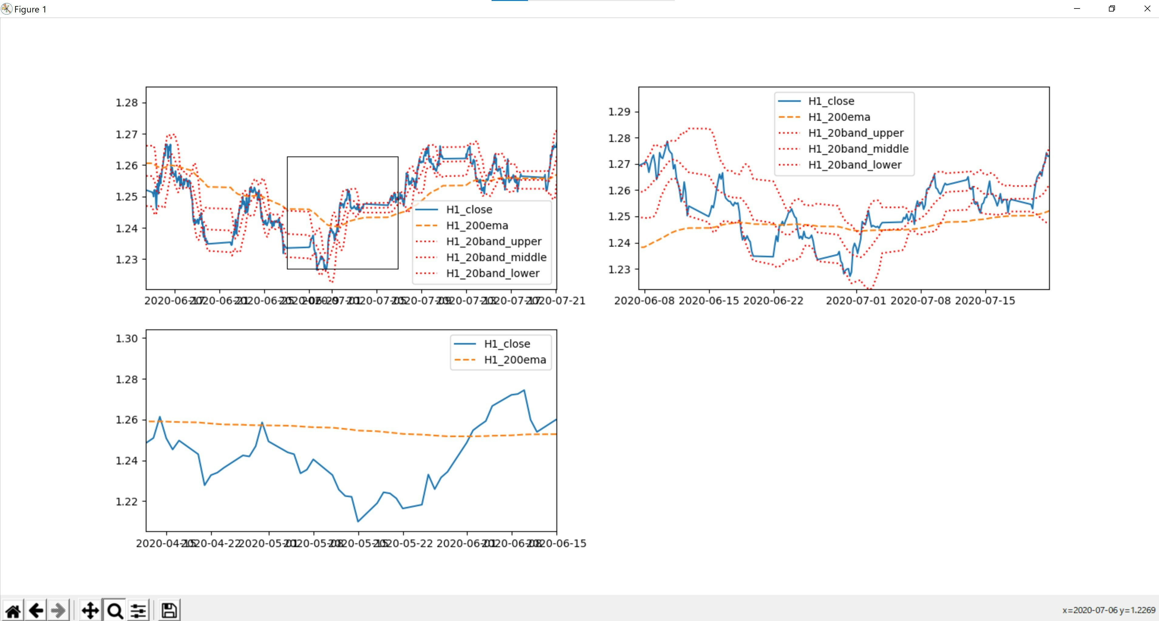
図3: 図2の左上の図の矩形選択部分を拡大。他2つの図に関しても同様の部分を拡大。

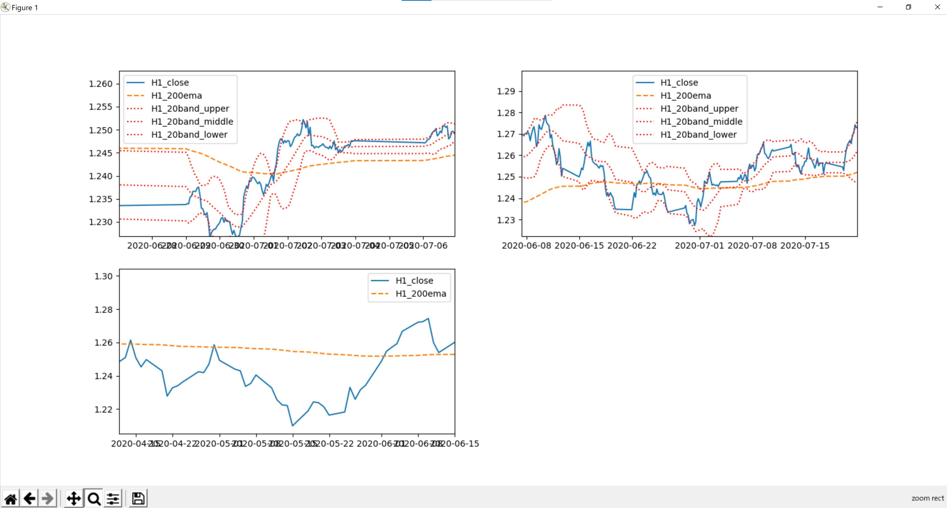
図4: 図3の左上の図の矩形選択部分を拡大。他2つの図に関しては図3から変化なし。

ソースコード

import MetaTrader5 as mt5
from datetime import datetime
from pytz import timezone
import numpy as np
import pandas as pd
import talib as ta
import matplotlib.pyplot as plt

def filterColumns(rates, dict_columns):
    """
    必要なカラムのみに絞り込む

    Parameters
    ---------
    rates : numpy.ndarray | pandas.DataFrame
        MT5から読み込んだデータ
    dict_columns : dictionary
        必要なカラム
        {置換前のカラム名1:置換後のカラム名1, 置換前のカラム名2:置換後のカラム名2, ...}

    Returns
    ---------
    df_rates : pandas.DataFrame
        必要なカラムのみに絞ったDataFrame
    """
    df_rates = pd.DataFrame(rates)
    df_rates['time'] = pd.to_datetime(df_rates['time'], unit='s')
    df_rates = df_rates.rename(columns=dict_columns)
    return_columns = ['time'] + list(dict_columns.values())
    return df_rates.loc[:, return_columns]

utc_tz = timezone('UTC')
pd.set_option('max_row', None)

###########################
# MT5からデータを取得
###########################
mt5.initialize()
EURJPY_D1_rates = mt5.copy_rates_range("GBPUSD", mt5.TIMEFRAME_D1, datetime(2019,6,12,0), datetime(2021,6,12,0))
EURJPY_H4_rates = mt5.copy_rates_range("GBPUSD", mt5.TIMEFRAME_H4, datetime(2019,6,12,0), datetime(2021,6,12,0))
EURJPY_H1_rates = mt5.copy_rates_range("GBPUSD", mt5.TIMEFRAME_H1, datetime(2019,6,12,0), datetime(2021,6,12,0))
mt5.shutdown()

###########################
# テクニカルデータの作成とデータの整形
###########################
# D1
# MT5から読み込んだデータをpandasのDataFrame型に変換
df_EURJPY_D1_rates = pd.DataFrame(EURJPY_D1_rates)
# TA-Libを使用して200EMAの値を算出し、DataFrameの新規カラムとして追加
df_EURJPY_D1_rates['ema'] = ta.EMA(df_EURJPY_D1_rates.close, timeperiod=200)
# 必要なカラムのみに絞り込み
df_EURJPY_D1_rates = filterColumns(df_EURJPY_D1_rates, {'close':'D1_close', 'ema':'D1_200ema'})

# H4
df_EURJPY_H4_rates = pd.DataFrame(EURJPY_H4_rates)
df_EURJPY_H4_rates['ema'] = ta.EMA(df_EURJPY_H4_rates.close, timeperiod=200)
df_EURJPY_H4_rates['upper_band'], df_EURJPY_H4_rates['middle_band'], df_EURJPY_H4_rates['lower_band'] = ta.BBANDS(df_EURJPY_H4_rates.close, timeperiod=20)
df_EURJPY_H4_rates = filterColumns(df_EURJPY_H4_rates, {'close':'H4_close', 'ema':'H4_200ema', 'upper_band':'H4_20band_upper', 'middle_band':'H4_20band_middle', 'lower_band':'H4_20band_lower'})

# H1
df_EURJPY_H1_rates = pd.DataFrame(EURJPY_H1_rates)
df_EURJPY_H1_rates['ema'] = ta.EMA(df_EURJPY_H1_rates.close, timeperiod=200)
df_EURJPY_H1_rates['upper_band'], df_EURJPY_H1_rates['middle_band'], df_EURJPY_H1_rates['lower_band'] = ta.BBANDS(df_EURJPY_H1_rates.close, timeperiod=20)
df_EURJPY_H1_rates = filterColumns(df_EURJPY_H1_rates, {'close':'H1_close', 'ema':'H1_200ema', 'upper_band':'H1_20band_upper', 'middle_band':'H1_20band_middle', 'lower_band':'H1_20band_lower'})

# H1のデータに対して右からH4, D1の順で日時データをキーとして結合
df_EURJPY_H4_D1_rates = pd.merge(df_EURJPY_H4_rates, df_EURJPY_D1_rates, on='time', how='outer')
df_EURJPY_H1_H4_D1_rates = pd.merge(df_EURJPY_H1_rates, df_EURJPY_H4_D1_rates, on='time', how='outer')

###########################
# 4650~4750行目を表示
# - 4686行目以前はデータが足りないためD1_200emaのデータは作られていない
###########################
print('\n---------------------------')
print('- GBPUSD rates')
print('- length: ', len(df_EURJPY_H1_H4_D1_rates))
print('---------------------------')
print(df_EURJPY_H1_H4_D1_rates[4650:4750])

# TODO H1がNaNとなる原因を調査する
# TODO H1がNaNとなっている行だけ日付順に並んでおらず、結合後のDataFrameの最後に纏められてしまう原因を調査する
# TODO H1がNaNの行は削除する

# CSVに出力
df_EURJPY_H1_H4_D1_rates.to_csv('20210613_0504.csv')

###########################
# チャートの描画設定
###########################
fig = plt.figure()

ax1 = fig.add_subplot(221)
ax2 = fig.add_subplot(222)
ax3 = fig.add_subplot(223)

ax1.plot(df_EURJPY_H1_rates.loc[:,'time'], df_EURJPY_H1_rates.loc[:,'H1_close'], linestyle = "solid", label = "H1_close")
ax1.plot(df_EURJPY_H1_rates.loc[:,'time'], df_EURJPY_H1_rates.loc[:,'H1_200ema'], linestyle = "dashed", label = "H1_200ema")
ax1.plot(df_EURJPY_H1_rates.loc[:,'time'], df_EURJPY_H1_rates.loc[:,'H1_20band_upper'], linestyle = "dotted", label = "H1_20band_upper", color = "red")
ax1.plot(df_EURJPY_H1_rates.loc[:,'time'], df_EURJPY_H1_rates.loc[:,'H1_20band_middle'], linestyle = "dotted", label = "H1_20band_middle", color = "red")
ax1.plot(df_EURJPY_H1_rates.loc[:,'time'], df_EURJPY_H1_rates.loc[:,'H1_20band_lower'], linestyle = "dotted", label = "H1_20band_lower", color = "red")
ax1.legend()

ax2.plot(df_EURJPY_H4_rates.loc[:,'time'], df_EURJPY_H4_rates.loc[:,'H4_close'], linestyle = "solid", label = "H1_close")
ax2.plot(df_EURJPY_H4_rates.loc[:,'time'], df_EURJPY_H4_rates.loc[:,'H4_200ema'], linestyle = "dashed", label = "H1_200ema")
ax2.plot(df_EURJPY_H4_rates.loc[:,'time'], df_EURJPY_H4_rates.loc[:,'H4_20band_upper'], linestyle = "dotted", label = "H1_20band_upper", color = "red")
ax2.plot(df_EURJPY_H4_rates.loc[:,'time'], df_EURJPY_H4_rates.loc[:,'H4_20band_middle'], linestyle = "dotted", label = "H1_20band_middle", color = "red")
ax2.plot(df_EURJPY_H4_rates.loc[:,'time'], df_EURJPY_H4_rates.loc[:,'H4_20band_lower'], linestyle = "dotted", label = "H1_20band_lower", color = "red")
ax2.legend()

ax3.plot(df_EURJPY_D1_rates.loc[:,'time'], df_EURJPY_D1_rates.loc[:,'D1_close'], linestyle = "solid", label = "H1_close")
ax3.plot(df_EURJPY_D1_rates.loc[:,'time'], df_EURJPY_D1_rates.loc[:,'D1_200ema'], linestyle = "dashed", label = "H1_200ema")
ax3.legend()

###########################
# チャートの描画
###########################
plt.show()