対人関係の可視化：facebook messengerで誰とやりとりしているかをRで

動機

誰かと仲良くなると急にメッセージが増える．そのあと疎遠になるとさっぱりやりとりをしなくなる傾向がある．いっぽう，長いあいだ関わりのある友人の場合，量は少ないが長期間にわたってメッセージをやりとりをする．こういうパターンを可視化したい．ひらたく言うと恋/友情/用事がどれほど熱くなって，どれくらいのスピードで冷めたかが見られるようになる．

データの収集

まずはfacebookからデータを引っ張ってこないと始まらない．Facebookにログインし，ページの右上からSettings>Download a copy of your Facebook data.と辿っていくと全データがダウンロードできる．人によっては数百MB，数GBにおよぶと思う．ZIPを解凍するとそこにhtml/messages.htmというファイルがある．ここに全メッセージのデータが入っている･･･はずだったのだが，最近仕様がかわったらしく../messages/フォルダに個々人にわかれて格納されている．こりゃ困った．

CSVにする

そこでいきなりRでないものを使ってCSVにまとめてもらう．
https://github.com/ownaginatious/fbchat-archive-parser
pipよくわかってないけどpipをできるようにするんや
ターミナルでpip install fbchat-archive-parserとしてから，上記のデータディレクトリのhtmlに移動してからfbcap ./messages.htm -f csvとすれば，その場にmessages.csvというファイルが生成される．

Rで可視化

まずはlibraries

library.r

library(tidyverse)
library(rstan)
library(plyr)  # for ddply, https://stackoverflow.com/questions/18379933/plotting-cumulative-counts-in-ggplot2
library(ggbeeswarm)
library(poweRlaw)
library(scales) # date_format
library(viridis)
library(ggridges)
library(extrafont)
library(lubridate)

インプット

input.r

data <- read_csv("input/20180221_messages.csv") 

data <- data %>%
  arrange(desc(date))
save(data, file = paste0("data/", Sys.Date(), "data.Rdata"))

dataを見てみるとthread, sender, date, messageと列がある．threadは会話のチャンク（？）で，senderは個々の発言者である．たとえばBarack Obama, Vladimir Putin, Xi Jinping氏とのグループ会話内でのPutinの発言であればthreadに"Barack Obama, Vladimir Putin, Xi Jinping"と表示され，senderには"Vladimir Putin"と表示される．

データの整形

まず上で保存したデータを読む．
load("data/2018-02-21data.Rdata")
データフレームを作る．

dataframe

df <- 
  data %>%
  filter(sender != my_name) %>% 
  filter(sender == thread) %>%
  # filter(date > Sys.Date() - 365) %>%
  ddply(.(sender), transform, total_count = length(date)) %>% 
  filter(total_count > mess_threshold) %>%
  arrange(desc(total_count)) %>%
  mutate(sender = as.factor(sender)) %>%
  as.tibble()

今回は自分の発言はどうでもいいのでmy_name = "Abe Shinzo"などとしておいて，senderがmy_nameである行をすべて除く．ただこのデータもたとえばあの「私が1のメッセージを送っているのに返事が0.358しかないじゃない！」みたいな使い方ができるので，そういう応用の場合はその場合で･･･
今回はプライベートなやりとりに限定したのでfilter(sender == thread)でグループ会話をすべて除いている．total_countは受信したメッセージの数．
そのデータを使って，わずかしかやりとりをしていない人たちを除く．
mess_threshold <- 200 # omit users with less than this amount of messages
ここで直近365日に限定してもよいのだがggplotでやったほうがよいので･･･ddplyのあたりはもっといい方法がありそう．arrange()は意味ないかも．

累積のメッセージ数の推移を可視化

プロット開始をたとえば留学から帰ってきた日，start_day <- "2014-07-01"とする．

cumulative_messages

df %>%
  ggplot(aes(x = date, color = sender)) + 
  geom_step(aes(total_count = total_count, y = ..y.. * total_count),
            stat = "ecdf") +
  scale_x_datetime(date_breaks = "1 year", date_labels = "%Y-%m",
                   limits = as.POSIXct(c(start_day, NA)),
                   expand = c(0,0)
  ) +
  scale_y_continuous(limits = c(1, NA), "total messages received") +
  theme_linedraw() +
  theme(text = element_text(family ="HiraKakuProN-W3"),
        # legend.position = "none"
  )

私の場合はこうなる．個人情報of個人情報なのでlegendのないバージョンで一部だけ･･･．

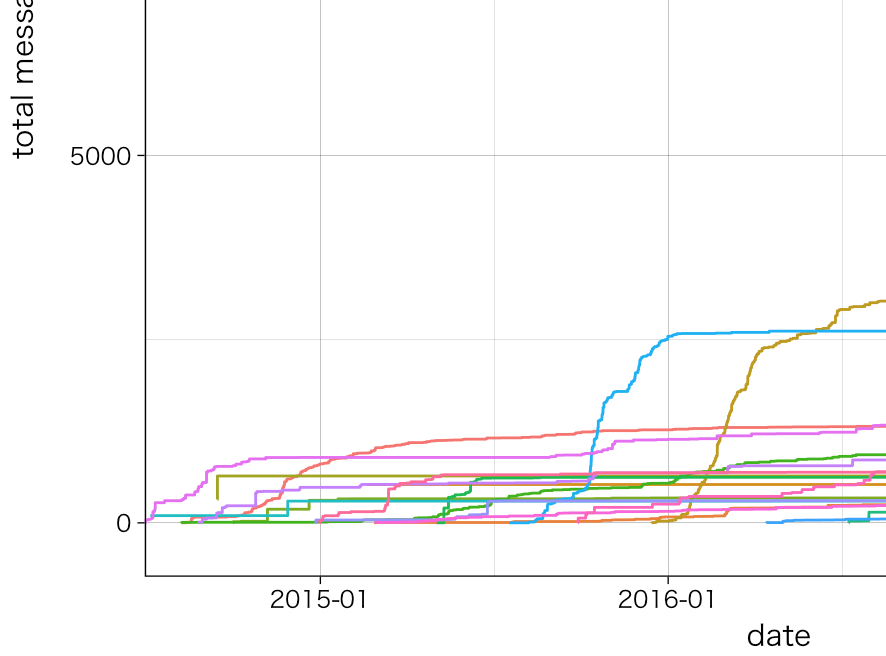
学習曲線的な，シグモイドな曲線が多い･･･．

個人のトレンド

このままではゴシャゴシャなので人に分けてみよう．最近violinplotよりbeeswarmより{ggbeeswarm}内のgeom_quasirandom()が良い感じで好きなのでこれを使う．色付けは{viridis}.

quasirandom

df %>%
  ggplot(aes(date, 
             y = reorder(x = sender, 
                         X = date,
                         FUN = min), 
             colour = date)) + # X = total_countにしてもよいと思う．
  geom_quasirandom(groupOnX = FALSE, 
                   size = 0.1, 
                   width = 0.95, # どれだけほかの人にかぶりかけるかdefault0.4
                   varwidth = TRUE, # 全体の大きさに応じてかわる
                   bandwidth = 0.2 # smoothness
  ) +
  geom_vline(xintercept = as.POSIXct(Sys.Date()), linetype = "longdash", size = 0.1) +
  scale_colour_viridis() + # もしcolourをsenderなどにするならdiscrete = TRUEを入れる
  scale_x_datetime(
    date_breaks = "1 year",
    labels = date_format("%Y-%m", tz = "Asia/Tokyo")
  ) +
  theme_light(12) +
  theme(
    legend.position = "none",
    aspect.ratio = 1
  ) 
ggsave(paste0("output/messenger_", Sys.Date(), "_beeswarm.pdf"), width = 250, height = 200, unit = "mm")

こうなる（一部）

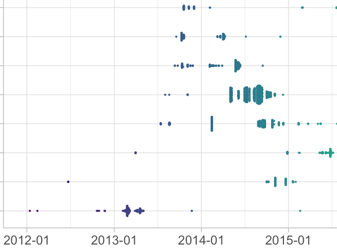
geom_quasirandom()にalpha = 0.03などをいれるとより綺麗だが見にくい．

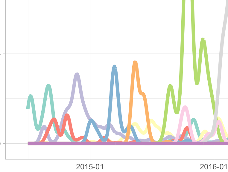
山脈状にする

上記とほぼ同じだが誰の山がいつきたか，その移行がどうなっているかは重ね書きしたほうがわかりやすい．

waves

# for tally (making the group "others") https://stackoverflow.com/questions/35113873/combine-result-from-top-n-with-an-other-category-in-dplyr
top_n_messengers <- 10
df <- 
  data %>%
  filter(sender != my_name) %>% 
  filter(sender == thread) %>%
  filter(date > start_day) %>%
  ddply(.(sender), transform, total_count = length(date)) %>%
  arrange(desc(total_count))
ranking <- 
  df %>% 
  group_by(sender) %>%
  tally(length(sender), sort = TRUE) 
ranking

df %>% 
  mutate(
    sender = ifelse(
      sender %in% ranking$sender[1:top_n_messengers],
      sender, NA
    )
  ) %>% 
  mutate(sender = as.factor(sender)) %>%
  as.tibble() %>%
  ggplot(aes(date, 
             y = ..count.., # to avoid accute ping
             colour = reorder(x = sender, 
                              X = date,
                              FUN = min)
  )) + 
  stat_density(
    geom = "line",
    size = 2,
    position = "identity", 
    bw = 800000) + # bwの値とかは場合に応じて変えたほうがいいかも
  geom_vline(xintercept = as.POSIXct(Sys.Date()), linetype = "longdash", size = 0.1) +
  scale_colour_brewer("sender", palette = "Set3") +
  # facet_grid(sender ~ .) +
  scale_x_datetime(
    date_breaks = "1 year",
    labels = date_format("%Y-%m", tz = "Asia/Tokyo")
  ) + 
  theme_light(12) +
  theme(
    legend.justification = c(0,1),
    legend.position = c(0.01,0.99)
  ) 
ggsave(paste0("output/messenger_", Sys.Date(), "_beeswarm.pdf"), width = 250, height = 200, unit = "mm")

こうなる

joyplot/ggridgesを使ってみる

さらに違う見方で

joyplot

df %>% 
  mutate(
    sender = ifelse(
      sender %in% ranking$sender[1:top_n_messengers],
      sender, NA
    )
  ) %>% 
  mutate(sender = as.factor(sender)) %>%
  as.tibble() %>%
  ggplot(aes(date, 
             y = reorder(x = sender, 
                         X = total_count),
             fill = NA,
             height = ..count..
  )) + 
  geom_density_ridges(
    bw = 0.001,
    # bins = 1000,
    colour = "white", 
    size = 0.2,
    scale = 2,
    # alpha = 0.7,
    rel_min_height = 0.0000000001,
    stat = "density"  # "binline"
  ) +
  geom_vline(xintercept = as.POSIXct(Sys.Date()), linetype = "longdash", size = 0.1) +
  # scale_fill_viridis(discrete = TRUE, option = "D") + # discrete = TRUE
  scale_fill_brewer("sender",
                    palette = "Set3") +
  # facet_grid(sender ~ .) +
  scale_x_datetime(
    date_breaks = "1 year",
    labels = date_format("%Y-%m", tz = "Asia/Tokyo")
  ) + # "2014-07-01"
  theme_linedraw() +
  theme(
    legend.position = "none",
    panel.background = element_rect(fill = "black"),
    # aspect.ratio = 
  ) 

トップ数人以外はothersに吸収させている．

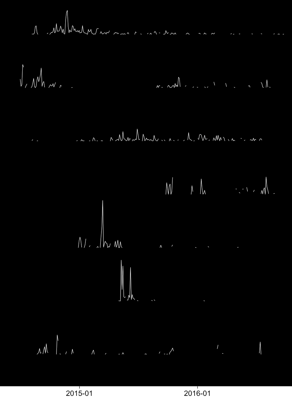
うーむかっこいい．誰が長く関わりを持っているかがよくわかる．

いつメッセージをやりとりしているか？

hour

data %>%
  filter(sender != my_name) %>% 
  filter(sender == thread) %>%
  filter(date > start_day) %>%
  ddply(.(sender), transform, total_count = length(date)) %>% 
  filter(total_count > mess_threshold) %>%
  arrange(desc(total_count)) %>%
  mutate(sender = as.factor(sender)) %>%
  as.tibble() %>%
  ggplot(
    aes(
      format(date, "%H:%M:%S") %>% 
        parse_date_time("HMS"),
      y = 0,
      # y = reorder(x = sender, 
      #             X = total_count),
      colour = sender
    )
  ) + # X = total_count
  # geom_density() +
  geom_quasirandom(groupOnX = FALSE,
                   size = 0.02,
                   width = 1, # どれだけほかの人にかぶりかけるかdefault0.4
                   varwidth = FALSE, # 全体の大きさに応じてかわる
                   # alpha = 0.1,
                   bandwidth = 0.05 # smoothness
  ) +
  scale_x_datetime(breaks = date_breaks("4 hour"),
                   labels = date_format("%H:%M", tz = "Asia/Tokyo")  # tz must be in here
  ) +
  coord_polar(theta = "x", 
              start = 2 * pi / 24 * 9 # time-zone offset of 9 hours
  ) +
  scale_y_continuous(limits = c(0, NA)) +
  facet_wrap(~sender) +
  theme_ridges(12) +
  scale_colour_viridis(option = "C",  discrete = TRUE) +
  theme(
    legend.position = "none"
  ) # https://stackoverflow.com/questions/7830022/rotate-x-axis-text-in-ggplot2-when-using-coord-polar

うまいやり方がわからなかったのでgeom_quasirandom()を無理やりcoord_polar()で丸めた．だいたい半分のデータが消えてしまうのでよくないと思うが趣味の可視化程度だったら別にいいのだ．tzのせいなのかなんなのか目盛りがよくわからないところから始まってしまうのも対処法がよくわからない．でも趣味の以下略

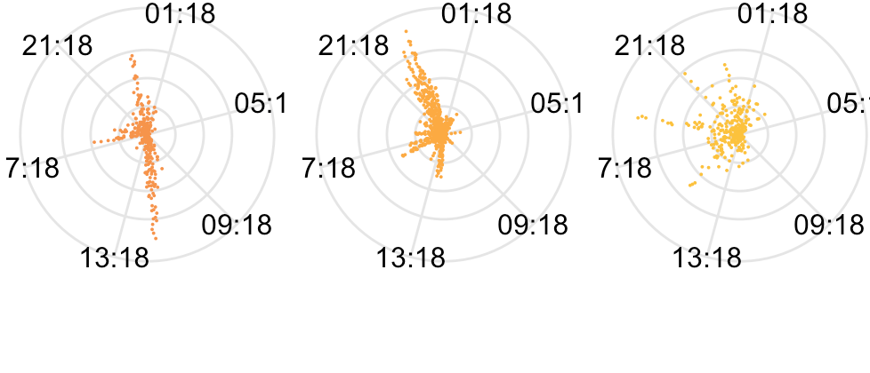
留学中にやりとりしていた人は日本時間の深夜にやり取りが多いかのように見える，あちらではそのあたりが日中なので．

おまけ：べき乗則

博士論文の内容とも関わるが，適当にメッセージする人を見繕って（variation），さらに次のタイムステップでランダムサンプルしたメッセージ（メッセージ相手ではない．メッセージ相手ごとにランダムサンプリングしたら指数分布に従うはずcf 2011 Mesoudi & Lycett）ようなモデルでも説明できそうだ．ひとまずxminは1に設定している．まぁ1でいいでしょ

powerlaw

aggr_data <- data %>%
  filter(sender == thread) %>% # avoid group conv
  group_by(sender) %>% 
  dplyr::summarise(count = n()) %>% 
  arrange(desc(count)) %>%
  filter(sender != my_name)

power_law <- displ$new(aggr_data$count)
log_normal <- dislnorm$new(aggr_data$count)
# power_law$setXmin(estimate_xmin(power_law))
power_law$setXmin(1)
log_normal$setXmin(1)
power_law$setPars(estimate_pars(power_law))
log_normal$setPars(estimate_pars(log_normal))
plot(power_law)
lines(power_law)
lines(log_normal)
df_pl <- plot(power_law)
df_pl2 <- left_join(aggr_data, df_pl, by = c("count" = "x"))
# latest message
last_date <- data %>% 
  group_by(sender) %>%
  filter(date == max(date)) %>% 
  distinct(sender, .keep_all = TRUE) # http://a-habakiri.hateblo.jp/entry/2016/11/29/215013 .を忘れず
# merge them
df_pl3 <- left_join(df_pl2, last_date, by = "sender")

ggplot(df_pl3, aes(count, y, colour = date)) +
  geom_point(size = 2) +
  # geom_text(check_overlap = FALSE, aes(label = sender), size = 1, 
  #           # position = position_jitter(width = 0.4, height = 0), 
  #           alpha = 0.8, 
  #           hjust = 0, nudge_x = 0.05
  #           ) +
  scale_x_continuous(trans = "log10", breaks = 10^(0:10))+
  scale_y_continuous(trans = "log10") +
  scale_colour_viridis(breaks = daybreak) + # discrete = TRUE
  theme_light() +
  theme(aspect.ratio = 1,
        # legend.position = "none"
  ) 
ggsave(paste0("output/messenger_", Sys.Date(), "_powerlaw.pdf"), width = 200, height = 150, unit = "mm")

私の場合こうなった．グラフの読み方に関してはClauset et al., 2009などを参考にしてください．power-lawではなくpower-law with exponential cut-offに見えるけど．でランダムモデルからの乖離したポイントの人があなたの特異な愛というわけ（適当）

Github

おしまい