誤り訂正学習

誤り訂正学習とは、機械にある事象について学習させることである。
その方法は様々だが今回は教師データをもとに学習する方法を簡単にプログラムして理解を試みる。
今回は中心が違う乱数データを機械学習によって教師信号と同じように分類するプログラムを書いた。

1　学習データの準備

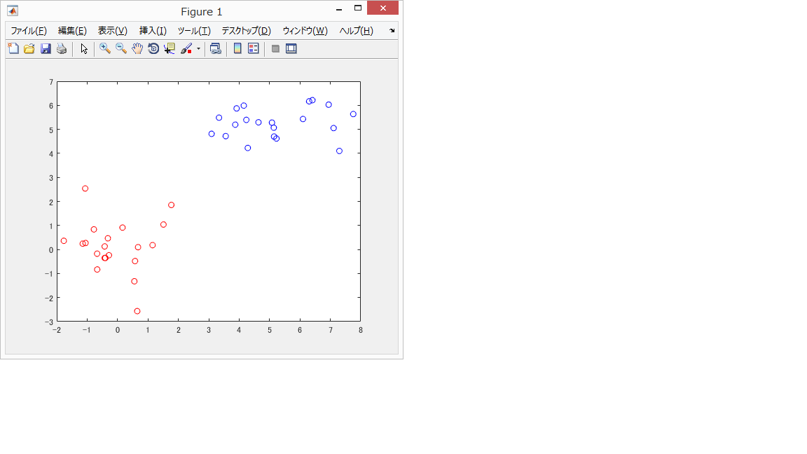
今回は座標平面上に(0,0)を中心とする点20個、(5,5)を中心とする点20個の計40個を使用する。
(0,0)を中心とする点を赤色、(5,5)を中心とする点を青色に出力し、教師信号とする。

% 2次元ベクトルinput1、20個、平均0、分散１、中心(0,0)
input1 = randn(20,2);
% 2次元ベクトルinput2、20個、平均0、分散１、中心(5,5)
input2 = randn(20,2)+5;
%望ましい出力
r=1;

% 1次元、2次元の値を各々-2から7までの範囲にて描画する
xlim([-2,7]);
ylim([-2,7]);
drawnow;

%出力
for i=1:20
  plot(input1(i,1),input1(i,2),'ro'); hold on;
  plot(input2(i,1),input2(i,2),'bo'); hold on;
end

2　学習前の状態

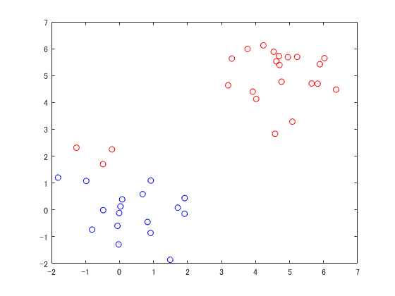
次に学習のプログラムを書かず、機械が適当に教会を決めるとどうなるかを試す。

結果
下に示すように教師信号とは全く別の場所が境界線となっていた。

% 2次元ベクトルinput1、20個、平均0、分散１、中心(0,0)
input1 = randn(20,2);
% 2次元ベクトルinput2、20個、平均0、分散１、中心(5,5)
input2 = randn(20,2)+5;
%二つのinputを合成
input0 = vertcat(input1,input2);
%しきい値をweights0とみなすためバイアスを設定
bias = 1;
% 重みを定義する
weights = randn(3,1);

% 入力より論理演算のorとして出力desired_outとして求める
for i = 1:40
% 識別関数をyで定義
y = bias * weights(1,1) + ...
    input0(i,1) * weights(2,1) + input0(i,2) * weights(3,1);
%yの計算結果を論理演算する
if y >= 0
    plot(input0(i,1),input0(i,2),'ro'); hold on;
else
    plot(input0(i,1),input0(i,2),'bo'); hold on;
end
end

% 1次元、2次元の値を各々-2から7までの範囲にて描画する
xlim([-2,7]);
ylim([-2,7]);
drawnow;

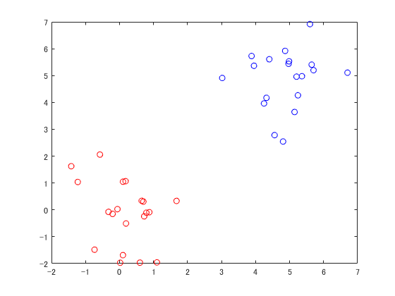
誤り訂正学習

最後に誤り訂正プログラムを書いて、教師信号道理に分類できているかを確かめる。

% 2次元ベクトルinput1、20個、平均0、分散１、中心(0,0)
input1 = randn(20,2);
% 2次元ベクトルinput2、20個、平均0、分散１、中心(5,5)
input2 = randn(20,2)+5;
%しきい値をweights0とみなすためバイアスを設定
bias = 1;
%二つのinputを合成
input0 = vertcat(input1,input2);
% 重み、しきい値を小さな数で定義する
weights = randn(3,1);

% 入力より論理演算のorとして出力desired_outとして求める
for i = 1:40
% 識別関数をyで定義
y = bias * weights(1,1) + ...
    input0(i,1) * weights(2,1) + input0(i,2) * weights(3,1);
%yの計算結果を論理演算する
if y >= 0
    output(i,1) = 1;
else
    output(i,1) = 0;
end
end

%学習回数を設定
interations=1000;
%学習効率aを設定
a=0.1;

for i= 1:interations
    % 出力ベクトルの値を0で初期化
     out = zeros(40,1);
    for j = 1:20
        r=1; %理想データr=1
        y =bias * weights(1,1) + ...
            input0(j,1) * weights(2,1) + input0(j,2) * weights(3,1);

        % 活性化関数にシグモイド関数を用い
        out(j) = 1/(1+exp(-y));
        % 解と出力の差を変数deltaとして求め
        delta = 1-out(j);

        %重みの更新
        weights(1,1)=weights(1,1)+a*delta*bias;
        weights(2,1)=weights(2,1)+a*delta*input0(j,1);
        weights(3,1)=weights(3,1)+a*delta*input0(j,2);
    end
    for j = 21:40
        r=0; %理想データ=0
        y =bias * weights(1,1) + ...
            input0(j,1) * weights(2,1) + input0(j,2) * weights(3,1);

        %理想データと出力の差
        % 活性化関数にシグモイド関数を用い
        out(j) = 1/(1+exp(-y));
        % 解と出力の差を変数deltaとして求め
        delta = 0-out(j);

        %重みの更新
        weights(1,1)=weights(1,1)+a*delta*bias;
        weights(2,1)=weights(2,1)+a*delta*input0(j,1);
        weights(3,1)=weights(3,1)+a*delta*input0(j,2);
    end
end

for i=1:40
% 識別関数をyを再計算
y = bias * weights(1,1) + ...
    input0(i,1) * weights(2,1) + input0(i,2) * weights(3,1);
 if y >= 0
  plot(input0(i,1),input0(i,2),'ro'); hold on;
 else
  plot(input0(i,1),input0(i,2),'bo'); hold on;
 end
end
hold on;

% 1次元、2次元の値を各々-2から7までの範囲にて描画する
xlim([-2,7]);
ylim([-2,7]);
drawnow;

まとめ

機械学習はもっと高度に発展していけるのでどんどん挑戦していきたい。