Udemy - ゼロからPythonで学ぶ人工知能と機械学習 : 数学系処理／ニューロン編

みんなのAI講座 ゼロからPythonで学ぶ人工知能と機械学習

パッケージインポート

Preferences or Setting -> [project name] -> Project Interpreter

• パッケージ追加不能の場合、packaging toolに関する警告が出ている場合それをインストール。
• matplotlib系のインポートにしくった。エラーテキストと格闘し、なんとか以下記事の方法で処理成功。
• http://zashikiro.hateblo.jp/entry/2012/10/02/130031
• https://stackoverflow.com/questions/44318333/unable-to-import-matplotlib-pyplot

一次関数プロット

• matplotlib, numpyのパッケージを使用する。
• pythonでは使用パッケージをエイリアス化可能な模様。

x = np.arange(0, 10, 0.1)   # 0〜9.9を0.1刻みで作ったものをリスト形式で格納
print x

y = 2 * x + 1 # xリストの各要素を二倍し、+1する
print y

plt.plot(x, y) # 作成したx,yで二次元グラフ描画
plt.show()

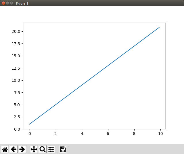
• plt.show()によりこんな感じのグラフが図表可能。このウィンドウ上で移動・拡大／縮小・範囲変更等可能。

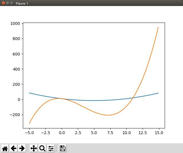
二次・三次関数同時プロット

• 式を作れば二次以上の関数も生成可能。
• 同一エイリアスに対し作った式を積んでいくことで同じグラフの中に描画する。

import matplotlib.pyplot as plt
import numpy as np

x = np.arange(-5, 15, 0.1)
print x

# 二次関数生成
# y = x^2 - 10x + 10
y_2 = x**2 - 10*x + 10
plt.plot(x, y_2)

# 三次関数生成
# y = x^3 - 10x^2 - 10x + 10
y_3 = x**3 - 10*x**2 - 10*x + 10
plt.plot(x, y_3)

# pltに放り込まれた関数を描画
plt.show()

シグモイド関数

• ユーザ定義関数で非引数・非ローカルの変数（この場合ネイピアe）は、外部スコープで定義されていれば問題ない？
• この場合はsigmoid(x)コール直前のeの値に従う？
• sigmoid(a)の中のeはどうせ定数なんだしmath.eでいいよなあと思う。
• Pythonのお作法的にどこでどう定義されているかわからない数を関数の中で使うのはアリなんだろうか。

def sigmoid(a):
    # y = 1 / (1 + e^(-1))
    s = 1 / (1 + e**-a)
    return s

e = math.e

dx = 0.1
x = np.arange(-8, 8, dx)
print x

y_sig = sigmoid(x)

plt.plot(x, y_sig)
plt.show()

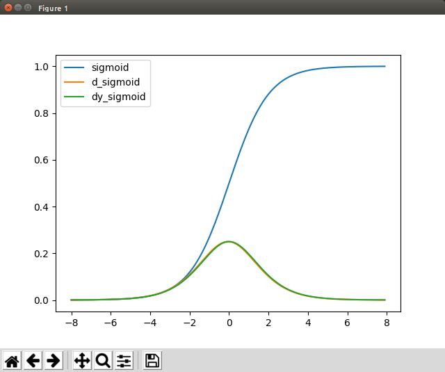
ラベル

• .plot時にlabel = "string"を付与し、.legendと合わせて使用すると描画グラフに名称が付く。

import matplotlib.pyplot as plt
import numpy as np
import math

def sigmoid(a):
    s = 1 / (1 + math.e**-a)
    return s

dx = 0.1
x = np.arange(-8, 8, dx)
print x

# シグモイド関数
y_sig = sigmoid(x)
# シグモイド関数の傾き算出
y_dsig = (sigmoid(x+dx) - sigmoid(x)) / dx
# シグモイド関数の微分
dy_sig = sigmoid(x) * (1 - sigmoid(x))

plt.plot(x, y_sig, label = "sigmoid")
plt.plot(x, y_dsig, label = "d_sigmoid")
plt.plot(x, dy_sig, label = "dy_sigmoid")
plt.legend()    # plot時にラベルを付与し、legendを呼び出すことで描画グラフに名称が付く
plt.show()

ニューラルネットワーク 入出力サンプル

• ニューロンを実装したニューラルネットワークのサンプル
• リストの数値を順次積んでいき、最終的に合計値が出る。
• 複数の入力から一つの出力を得る。

# Neuron class
class Neuron :
    input_sum = 0.0 # 最終的にこの値が少しずつ増える
    output = 0.0    # output用

    def setInput(self, inp):
        self.input_sum += inp

    def getOutput(self):
        self.output = self.input_sum
        return self.output

# Neural Newrok class
class NeuralNetwork:
    # Create Neuron instance
    neuron = Neuron()
    # Receive inputs,
    def commit(self, input_data):
        for data in input_data:
            # setInputメソッドに各入力を与えていく
            self.neuron.setInput(data)
        return self.neuron.getOutput()

# Create NeuralNework instance
neural_network = NeuralNetwork()

# Execute
trial_data = [1.0, 2.0, 3.0]
print "Output =", neural_network.commit(trial_data)

実行結果

Output = 6.0

ニューラルネットワーク 単一ニューロンサンプル

• だんだんわかりにくくなってきた。
• シグモイド関数からの出力は$ \frac{1}{1 + e^{-x}} $で得る。
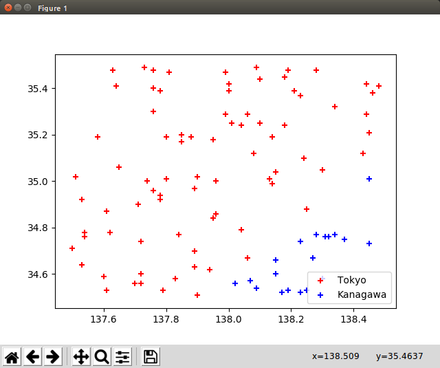
• 一地点における「入力」は緯度(λ)・経度(θ)・バイアス値(b)となり、「出力」の値を得る。
• 今回の場合は $ sigmoid(\lambdaw_0 + \thetaw_1 + b*w_2) $ の値が出力値となり、0.5を閾値として東京／神奈川を判断する。
• シグモイドへの入力値が大きすぎる／小さすぎると上手く学習できないため、入力が0.0〜1.0の範囲に収まるよう基準点のオフセットrefer_point_0/1を使い、ニューロンへの入力値を補正し、グラフ描画時に戻している。

# coding: UTF-8
import matplotlib.pyplot as plt
import math

# シグモイド関数定義
def sigmoid(a):
    # math.exp(-a) = e^-1
    return (1.0 / (1.0 + math.exp(-a)))

# Neuron class
class Neuron :
    input_sum = 0.0 # 最終的にこの値が少しずつ増える
    output = 0.0    # output用

    def setInput(self, inp):
        self.input_sum += inp

    def getOutput(self):
        self.output = sigmoid(self.input_sum)
        return self.output

    # input/output values intialize
    def reset(self):
        self.input_sum = 0
        self.output = 0

# Neural Newrok class
class NeuralNetwork:
    # 入力値の重みづけ
    w = [-0.5, 0.5, -0.2] # [2]はバイアス重み
    # Create Neuron instance
    neuron = Neuron()
    # Receive inputs,
    def commit(self, input_data):
        self.neuron.reset()

        bias = 1.0
        self.neuron.setInput(input_data[0] * self.w[0])
        self.neuron.setInput(input_data[1] * self.w[1])
        self.neuron.setInput(bias * self.w[2])
        return self.neuron.getOutput()

# 基準点(データの範囲を0.0〜1.0内に収める為)
refer_point_0 = 34.5
refer_point_1 = 137.5

# Read data
i = 0
trial_data = []
trial_data_file = open("trial_data.txt", "r")
for line in trial_data_file:
    i += 1
    line = line.rstrip().split(",") # 改行を取り除き,で分ける
    # print (float(line[0]) - refer_point_0), (float(line[1]) - refer_point_1)
    trial_data.append([float(line[0]) - refer_point_0, float(line[1]) - refer_point_1])
trial_data_file.close()

# Create NeuralNework instance
neural_network = NeuralNetwork()

# Execute
position_tokyo = [[], []] # [経度, 緯度]
position_kanagawa = [[], []] # [経度, 緯度]
for data in trial_data:
    # cmt = sigmoid(data[0] + data[1])
    cmt = neural_network.commit(data)
    print data[0], data[1],
    print '{:.2f}'.format(cmt),
    if cmt < 0.5:
        print "TKO"
        position_tokyo[0].append(data[1] + refer_point_1)  # add 経度
        position_tokyo[1].append(data[0] + refer_point_0)  # add 緯度
    else:
        print "KNGW"
        position_kanagawa[0].append(data[1] + refer_point_1)  # add 経度
        position_kanagawa[1].append(data[0] + refer_point_0)  # add 緯度

# trial_data = [1.0, 2.0, 3.0]
# print "Output =", neural_network.commit(trial_data)
# 合計値が0の時は0.5、正方向に増えると１に漸近、小さくなると０に漸近

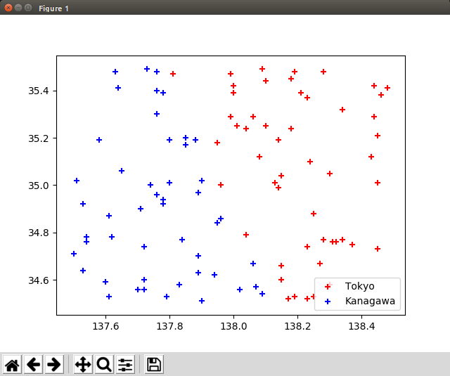
# 散布図描画
plt.scatter(position_tokyo[0], position_tokyo[1], c = "red", label = "Tokyo", marker = "+")
plt.scatter(position_kanagawa[0], position_kanagawa[1], c = "blue", label = "Kanagawa", marker = "+")
plt.legend()
plt.show()

ニューラルネットワーク 三層ネットワークサンプル（教師なし）

• 入力層・中間層・出力層の三層で構成する。
  
• サクッと書いたものなので適当なのはご勘弁。
• 入力層の各ニューロン（およびバイアス）の出力が、中間層の各ニューロンへの入力となる。
• 同じように中間層各ニューロン（およびバイアス）の出力が、出力層ニューロンへの入力となる。
• ニューロン間の出入力には規定の重みが乗算される。
• 最終ニューロンの出力がネットワーク全体の出力となる。

# coding: UTF-8
import matplotlib.pyplot as plt
import math

# シグモイド関数定義
def sigmoid(a):
    # math.exp(-a) = e^-1
    return (1.0 / (1.0 + math.exp(-a)))

# Neuron class
class Neuron :
    input_sum = 0.0 # 最終的にこの値が少しずつ増える
    output = 0.0    # output用

    def setInput(self, inp):
        self.input_sum += inp

    def getOutput(self):
        self.output = sigmoid(self.input_sum)
        return self.output

    # input/output values intialize
    def reset(self):
        self.input_sum = 0
        self.output = 0

# Neural Newrok class
class NeuralNetwork:
    # 入力値の重みづけ
    # 入力層・中間層間の重み
    w_im = [[0.496, 0.512], [-0.501, 0.998], [0.498, -0.502]] # 第一入力NEU→各中間NEUの重み, 第二入力NEU→各中間NEUの重み, 入力バイアス→各中間NEUの重み
    # 中間層・出力層間の重み
    w_mo = [0.121, -0.4996, 0.200] # 第一中間NEU→出力NEUの重み, 第二中間NEU→出力NEUの重み, 中間バイアス→出力NEUの重み

    # 入力層：N（ニューロン）、N、バイアス　入力層は数値がそのまま入る
    input_layer = [0.0, 0.0, 1.0]
    # 中間層：Nインスタンス、Nインスタンス、バイアス
    middle_layer = [Neuron(), Neuron(), 1.0]
    # Nはひとつだけ
    output_layer = Neuron()

    # Receive inputs,
    def commit(self, input_data):
        # 各層ニューロン初期化
        self.input_layer[0] = input_data[0]
        self.input_layer[1] = input_data[1]
        self.middle_layer[0].reset()
        self.middle_layer[1].reset()
        self.output_layer.reset()

        # 入力層→中間層
        # 第一中間ニューロンに入力３つ
        nr_idx = 0
        self.middle_layer[nr_idx].setInput(self.input_layer[0] * self.w_im[0][nr_idx]) # 第一入力N出力値×対応重み
        self.middle_layer[nr_idx].setInput(self.input_layer[1] * self.w_im[1][nr_idx])
        self.middle_layer[nr_idx].setInput(self.input_layer[2] * self.w_im[2][nr_idx]) # バイアス

        # 第二中間ニューロンに入力３つ
        nr_idx = 1
        self.middle_layer[nr_idx].setInput(self.input_layer[0] * self.w_im[0][nr_idx])
        self.middle_layer[nr_idx].setInput(self.input_layer[1] * self.w_im[1][nr_idx])
        self.middle_layer[nr_idx].setInput(self.input_layer[2] * self.w_im[2][nr_idx]) # バイアス

        # 中間層→出力層
        self.output_layer.setInput(self.middle_layer[0].getOutput() * self.w_mo[0])
        self.output_layer.setInput(self.middle_layer[1].getOutput() * self.w_mo[1])
        self.output_layer.setInput(self.middle_layer[2] * self.w_mo[2]) # バイアス

        return self.output_layer.getOutput() # ニューラルネットワーク全体の出力値が帰る

# 基準点(データの範囲を0.0〜1.0内に収める為)
refer_point_0 = 34.5
refer_point_1 = 137.5

# Read data
i = 0
trial_data = []
trial_data_file = open("trial_data.txt", "r")
for line in trial_data_file:
    i += 1
    line = line.rstrip().split(",") # 改行を取り除き,で分ける
    # print (float(line[0]) - refer_point_0), (float(line[1]) - refer_point_1)
    trial_data.append([float(line[0]) - refer_point_0, float(line[1]) - refer_point_1])
trial_data_file.close()

# Create NeuralNework instance
neural_network = NeuralNetwork()

# Execute
position_tokyo = [[], []] # [経度, 緯度]
position_kanagawa = [[], []] # [経度, 緯度]
for data in trial_data:
    # cmt = sigmoid(data[0] + data[1])
    cmt = neural_network.commit(data)
    print data[0], data[1],
    print '{:.2f}'.format(cmt),
    if cmt < 0.5:
        print "TKO"
        position_tokyo[0].append(data[1] + refer_point_1)  # add 経度
        position_tokyo[1].append(data[0] + refer_point_0)  # add 緯度
    else:
        print "KNGW"
        position_kanagawa[0].append(data[1] + refer_point_1)  # add 経度
        position_kanagawa[1].append(data[0] + refer_point_0)  # add 緯度

# 散布図描画
plt.scatter(position_tokyo[0], position_tokyo[1], c = "red", label = "Tokyo", marker = "+")
plt.scatter(position_kanagawa[0], position_kanagawa[1], c = "blue", label = "Kanagawa", marker = "+")
plt.legend()
plt.show()