A Probabilistic Trading Strategy on SmartTrade

In the last 3 articles, we illustrated 3 different trading strategies using various methodologies including ta-lib and statsmodel. In this article, we will explore the use of probabilistic approach to generate trading signals. Below assumes you already know the basics on how to create a trading strategy on SmartTrade. If not, please read the previous articles first.

Probabilistic vs. Rule-Based Approach

Up until now, we have been using a rule-based approach on our last trading strategies. For example, a "rule" to go long a stock if RSI < 30, or if price is below Bollinger Band for 2 days in a row, etc.. In other words, a "if logic" based on empirical study of past prices, generally on the premise that if certain conditions happen (e.g. oversold or strong momentum), then most likely prices will continue to go higher, and hence triggering a buy signal.

On the other hand, probabilistic approach bases its decision on the probability distribution on price data of a stock. Specifically, we issue a buy signal if distribution shows a high probability given past prices and vice-versa for sell signal.

Below we will illustrate an example on creating a trading strategy using a probabilistic approach with 2 steps .

1. Creating a Probability Distribution

Firstly, we define a learning period of which we will use to create a probability distribution. In our example, we will use the first 1000 trading days from 2007 as the learning period.

Then, we create our probability distribution functions based on the "return streak", which is the # of days up or down in a row. In SmartTrade, here is the code to do the above:

for (sym,val) in close.items():
          f = [0 for x in range(-50,50)]
          fn = [ 0 for x in range(-50,50)]
          pn = [ 0 for x in range(-50,50)]
          test = np.sign( val.values[1:] - val.values[:-1] )
          n = len(test)
  
          for i, row in enumerate(test):
            result[sym][i+1] = 0 if isNaN(test[i]) else (test[i] + ( 0 if test[i] != test[i-1] else result[sym][i] ) )
            if ( i < 1000 ):
              f[ result[sym][i+1] ] += val[i+5] / val[i] - 1
              fn[result[sym][i+1] ] += 1 
              pn[result[sym][i+1] ] += 1 if val[i+5] > val[i] else 0 

The key variables are f, fn and pn which store the results of the probability distribution based on the return streak (variable result):

• f is the average posterier 5-day return
• fn is the total number of occurences
• pn is the total number of occurences with positive 5-day return

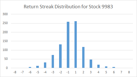
For example, here is the graph of fn for a particular stock:

The x-axis shows the return streak (days up or down in a row). The more negative, the longer the down streak is, and vice versa. The y-axis shows number of occurences given a particular streak #. The graph has a bell curve shape as expected, with most occurences in the middle which make sense as the likelihood a stock goes up or down decreases as the positive or negative streak increases.

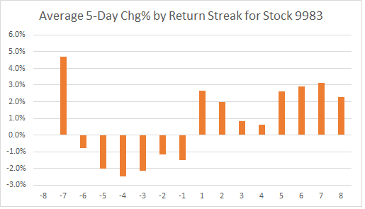
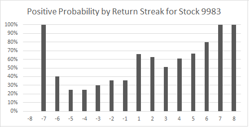
Next, we want to understand the return behavior given the streak #. We graph the average 5-day return (f) and positive probability (pn/fn) as follows:

As an example on how to interpret the results, we look at return streak of 5 (up 5 days in a row). We can see the average 5-day return is +2.5% with a positive probability of 65%. In other words, when the stock is up 5 days in a row, there is a 65% chance the stock will be up the next 5 days with a average gain of 2.5%.

1. Constructing Buy/Sell Signal

Given the above calculations, we will create buy and sell signals with these conditions on the backtesting period (after 1000 days):

• Buy if average 5 day return > +1% and if positive probability > 60%
• Sell if average 5 day return < 0% and if positive probability < 40%

 for i in range(1000,len(result[sym]) ):
       if f[result[sym][i]] > 0.01 and pn[result[sym][i]] / fn[result[sym][i]] > 0.6 :
          result2[ sym ][ i ] = 1  
       elif f[result[sym][i]] < 0 and pn[result[sym][i]] / fn[result[sym][i]] <0.4 :
          result2[ sym ][ i ] = -1 

buy_sig = result2[ (result2>0 )     ]
sell_sig = result2[  (result2<0) ]

Backtesting Result of Probabilistic Trading Strategy

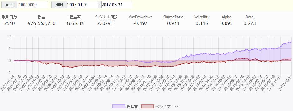
We applied the above strategy to 50 random stocks and below is the backtesting result on SmartTrade. Note that because the first 1000 days is the learning period, the return is zero until 2011, when the learning period ends and the actual backtesting period begins. As can be seen, the return metrics are solid comparing to the Nikkei 225 benchmark.

In conclusion, probabilistic approach has many advantages such as its flexibility to learn from different indicators, and can be easily expanded to self-learn over time. On the other hand, it requires a learning period which means more data is required for the method to be robust.

For full code, please see https://beta.smarttrade.co.jp/demo/7f12e5aa016d4c04b74641fe18c544ff