はじめに
自分用です. なんとなく気になったので.
それぞれの機械学習モデルが変数同士の和と積を認識できるか調べました.
線形回帰, サポートベクターマシン, 決定木, ランダムフォレスト, 全結合ニューラルネットワーク, LightGBMについて調べました.
2/13追記: 画像がリンク切れになっているので時間のある時に直します。
3/21追記: 直しました
雰囲気でゆるくやったのでハイパーパラメータ設定には特に力を入れていませんし, 厳密さは欠けているかもしれません.
データセット
3000行あります.
列a, b: -50から50のランダムな整数値(ExcelのRANDBETWEEN関数を使用)
列a+b: aとbの和
列a*b: aとbの積
| a | b | a+b | a*b | |
|---|---|---|---|---|
| 0 | 37 | 46 | 83 | 1702 |
| 1 | -30 | 35 | 5 | -1050 |
| 2 | -19 | 46 | 27 | -874 |
| 3 | 14 | 26 | 40 | 364 |
| 4 | 3 | -10 | -7 | -30 |
各機械学習モデルにおける実験
訓練データとテストデータに分けます.
8:2で分けるので訓練データは2400個のデータを持ちます.
train, test = train_test_split(df,test_size = 0.2,random_state = 42)
X_train = train.iloc[:,:2]
y1_train = train.iloc[:,2]
y2_train = train.iloc[:,3]
X_test = test.iloc[:,:2]
y1_test = test.iloc[:,2]
y2_test = test.iloc[:,3]
ここから先ではこのデータを機械学習モデルに入力し, RMSEやMAEを使って評価します.
a+b(和) -> a*b(積)の順に実行します.
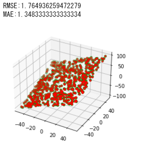
グラフは緑が正解データ, 赤が予測データを示します.
線形回帰
a+b
from sklearn.linear_model import LinearRegression
reg = LinearRegression()

reg.fit(X_train, y1_train)
y1_pred = reg.predict(X_test)

print("切片=", reg.intercept_, "回帰係数=", reg.coef_)
print(f'RMSE:{np.sqrt(mean_squared_error(y1_test, y1_pred))}')
print(f'MAE:{mean_absolute_error(y1_test, y1_pred)}')

fig = plt.figure()
ax = fig.add_subplot(projection='3d')
ax.scatter(X_test.iloc[:,0], X_test.iloc[:,1], y1_test, color='green') #s=20
ax.scatter(X_test.iloc[:,0], X_test.iloc[:,1], y1_pred, color='red', s=10)
plt.show()
 切片がほぼ0, 回帰係数は[1, 1]になっているので, a+bをうまく捉えているようです.
RMSEやMAEもほぼ0になりました.
切片がほぼ0, 回帰係数は[1, 1]になっているので, a+bをうまく捉えているようです.
RMSEやMAEもほぼ0になりました.
a*b
reg = LinearRegression()
reg.fit(X_train, y2_train)

y2_pred =reg.predict(X_test)
print("切片=", reg.intercept_, "回帰係数=", reg.coef_)
print(f'RMSE:{np.sqrt(mean_squared_error(y2_test, y2_pred))}')
print(f'MAE:{mean_absolute_error(y2_test, y2_pred)}')

fig = plt.figure()
ax = fig.add_subplot(projection='3d')
ax.scatter(X_test.iloc[:,0], X_test.iloc[:,1], y2_test, color='green')
ax.scatter(X_test.iloc[:,0], X_test.iloc[:,1], y2_pred, color='red', s=10)
plt.show()

予測した関数は平面状になってます. これは線形回帰のモデル上仕方ないことであり, 線形回帰で非線形関数を表現することはできないことがわかります.
サポートベクターマシン
a+b
from sklearn import svm
svc = svm.SVC(gamma="scale")
svc.fit(X_train, y1_train)

y1_pred = svc.predict(X_test)

print(f'RMSE:{np.sqrt(mean_squared_error(y1_test, y1_pred))}')
print(f'MAE:{mean_absolute_error(y1_test, y1_pred)}')

fig = plt.figure()
ax = fig.add_subplot(projection='3d')
ax.scatter(X_test.iloc[:,0], X_test.iloc[:,1], y1_test, color='green')
ax.scatter(X_test.iloc[:,0], X_test.iloc[:,1], y1_pred, color='red', s=10)
plt.show()

線形回帰ほどではないですが, 和を表現できているように見えます.
今回はハイパーパラメータをほとんど調整してないので, やろうと思えばもう少し誤差を減らせるかもしれません.
a*b
svc = svm.SVC(gamma="scale")
svc.fit(X_train, y2_train)

y2_pred = svc.predict(X_test)
print(f'RMSE:{np.sqrt(mean_squared_error(y2_test, y2_pred))}')
print(f'MAE:{mean_absolute_error(y2_test, y2_pred)}')

fig = plt.figure()
ax = fig.add_subplot(projection='3d')
ax.scatter(X_test.iloc[:,0], X_test.iloc[:,1], y2_test, color='green')
ax.scatter(X_test.iloc[:,0], X_test.iloc[:,1], y2_pred, color='red', s=10)
plt.show()

平面が歪んで正解値に近づいている感じになりました.
決定木
a+b
from sklearn.tree import DecisionTreeRegressor
dtr = DecisionTreeRegressor()
dtr.fit(X_train, y1_train)

y1_pred = svc.predict(X_test)

print(f'RMSE:{np.sqrt(mean_squared_error(y1_test, y1_pred))}')
print(f'MAE:{mean_absolute_error(y1_test, y1_pred)}')

fig = plt.figure()
ax = fig.add_subplot(projection='3d')
ax.scatter(X_test.iloc[:,0], X_test.iloc[:,1], y1_test, color='green')
ax.scatter(X_test.iloc[:,0], X_test.iloc[:,1], y1_pred, color='red', s=10)
plt.show()
a*b
dtr = DecisionTreeRegressor()
dtr.fit(X_train, y2_train)

y2_pred = dtr.predict(X_test)
print(f'RMSE:{np.sqrt(mean_squared_error(y2_test, y2_pred))}')
print(f'MAE:{mean_absolute_error(y2_test, y2_pred)}')

fig = plt.figure()
ax = fig.add_subplot(projection='3d')
ax.scatter(X_test.iloc[:,0], X_test.iloc[:,1], y2_test, color='green')
ax.scatter(X_test.iloc[:,0], X_test.iloc[:,1], y2_pred, color='red', s=10)

plt.show()

かなり精度よく近似できています. 木構造は分岐の繰り返しで和や積の相互作用を認識できるようで, その結果が表れています.
ランダムフォレスト
a+b
from sklearn.ensemble import RandomForestRegressor
rfg = RandomForestRegressor(n_jobs=-1, random_state=2525)
rfg.fit(X_train, y1_train)

y1_pred = rfg.predict(X_test)

print(f'RMSE:{np.sqrt(mean_squared_error(y1_test, y1_pred))}')
print(f'MAE:{mean_absolute_error(y1_test, y1_pred)}')

fig = plt.figure()
ax = fig.add_subplot(projection='3d')
ax.scatter(X_test.iloc[:,0], X_test.iloc[:,1], y1_test, color='green')
ax.scatter(X_test.iloc[:,0], X_test.iloc[:,1], y1_pred, color='red', s=10)

plt.show()

a*b
rfg = RandomForestRegressor(n_jobs=-1, random_state=2525)
rfg.fit(X_train, y2_train)

y2_pred =rfg.predict(X_test)
print(f'RMSE:{np.sqrt(mean_squared_error(y2_test, y2_pred))}')
print(f'MAE:{mean_absolute_error(y2_test, y2_pred)}')

fig = plt.figure()
ax = fig.add_subplot(projection='3d')
ax.scatter(X_test.iloc[:,0], X_test.iloc[:,1], y2_test, color='green')
ax.scatter(X_test.iloc[:,0], X_test.iloc[:,1], y2_pred, color='red', s=10)

plt.show()

決定木が相互作用を認識できるのでその発展モデルであるランダムフォレストも認識しています. 誤差はこちらの方が小さくなりました.
全結合ニューラルネットワーク
2->32->16->1の全結合層を持つ全結合層ニューラルネットワークです.
活性化関数はReluを使っています.
最適化手法はRMSProp, 誤差関数はMSELoss.
バッチサイズ100でa+bは1000エポック, a*bは2000エポック学習を行っています.
a+b
class DefineNN(nn.Module):
    def __init__(self):
        super().__init__()
        self.layers = nn.Sequential(
            nn.Linear(2,32),
            nn.ReLU(inplace=True),
            nn.Linear(32,16),
            nn.ReLU(inplace=True),
            nn.Linear(16,1),
        )

    def forward(self, x):
        return self.layers(x)

device = torch.device('cuda' if torch.cuda.is_available() else 'cpu')
model = DefineNN().to(device)

optimizer = torch.optim.RMSprop(model.parameters(), lr=0.01)
criterion = nn.MSELoss()

X_train = X_train.astype('float32')
X_test = X_test.astype('float32')
y1_train = y1_train.astype('float32')
y1_test = y1_test.astype('float32')
y2_train = y2_train.astype('float32')
y2_test = y2_test.astype('float32')

X_trainT = torch.tensor(X_train.values)
X_testT = torch.from_numpy(X_test.values)
y1_trainT = torch.from_numpy(y1_train.values)#.type(torch.LongTensor)
y1_testT = torch.from_numpy(y1_test.values)#.type(torch.LongTensor)
y2_trainT = torch.from_numpy(y2_train.values)#.type(torch.LongTensor)
y2_testT = torch.from_numpy(y2_test.values)#.type(torch.LongTensor)

batch_size = 100
num_epochs = 1000

train = torch.utils.data.TensorDataset(X_trainT,y1_trainT)
validation = torch.utils.data.TensorDataset(X_testT,y1_testT)
train_loader = DataLoader(train, batch_size = batch_size, shuffle = False)
validation_loader = DataLoader(validation, batch_size = batch_size, shuffle = False)

import time
print('start')
epoch_loss = []
for epoch in range(num_epochs):
    epoch_start_time = time.time()
    for x, y in train_loader:
        x = x.to(device)
        y = y.to(device)

        optimizer.zero_grad()
        outputs = model(x)
        loss = criterion(outputs.reshape(-1), y)
        loss.backward()
        optimizer.step()

    epoch_loss.append(loss.data.numpy().tolist())
    if (epoch+1)%100 == 0:
        print(f"Epoch: {epoch+1}/{num_epochs}.. ",
              f"Time: {time.time()-epoch_start_time:.2f}s..",
              f"Training Loss: {loss:.3f}.. ",)
print('fin')
start
Epoch: 100/1000.. Time: 0.03s.. Training Loss: 0.040..
Epoch: 200/1000.. Time: 0.04s.. Training Loss: 0.068..
Epoch: 300/1000.. Time: 0.03s.. Training Loss: 0.002..
Epoch: 400/1000.. Time: 0.03s.. Training Loss: 0.638..
Epoch: 500/1000.. Time: 0.03s.. Training Loss: 0.084..
Epoch: 600/1000.. Time: 0.03s.. Training Loss: 0.008..
Epoch: 700/1000.. Time: 0.03s.. Training Loss: 0.005..
Epoch: 800/1000.. Time: 0.04s.. Training Loss: 0.021..
Epoch: 900/1000.. Time: 0.03s.. Training Loss: 0.004..
Epoch: 1000/1000.. Time: 0.03s.. Training Loss: 0.031..
fin
fig = plt.figure()
ax = fig.add_subplot()
ax.plot(list(range(len(epoch_loss))), epoch_loss)
ax.set_xlabel('#epoch')
ax.set_ylabel('loss')
fig.show()

誤差が振動しつつ0に近づいてます.
print(f'RMSE:{np.sqrt(mean_squared_error(Y1, y1_pred))}')
print(f'MAE:{mean_absolute_error(Y1, y1_pred)}')

fig = plt.figure()
ax = fig.add_subplot(projection='3d')
ax.scatter(X.iloc[:,0], X.iloc[:,1], Y1, color='green', s=10)
ax.scatter(X.iloc[:,0], X.iloc[:,1], y1_pred, color='red', s=5)

plt.show()

かなり精度よく近似できました.
a*b
model = DefineNN().to(device)
optimizer = torch.optim.RMSprop(model.parameters(), lr=0.01)
criterion = nn.MSELoss()

train = torch.utils.data.TensorDataset(X_trainT,y2_trainT)
validation = torch.utils.data.TensorDataset(X_testT,y2_testT)
train_loader = DataLoader(train, batch_size = batch_size, shuffle = False)
validation_loader = DataLoader(validation, batch_size = batch_size, shuffle = False)

print('start')
epoch_loss = []
model.train()

i=2
num_epochs = 1000*i #epochを増やした

for epoch in range(num_epochs):
    epoch_start_time = time.time()
    for x, y in train_loader:
        x = x.to(device)
        y = y.to(device)

        optimizer.zero_grad()
        outputs = model(x)
        loss = criterion(outputs.reshape(-1), y)
        loss.backward()
        optimizer.step()

    epoch_loss.append(loss.data.numpy().tolist())
    if (epoch+1)%100 == 0:
        print(f"Epoch: {epoch+1}/{num_epochs}.. ",
              f"Time: {time.time()-epoch_start_time:.2f}s..",
              f"Training Loss: {loss:.3f}.. ",)
print('fin')
start
Epoch: 100/2000.. Time: 0.03s.. Training Loss: 7051.329..
Epoch: 200/2000.. Time: 0.03s.. Training Loss: 602.597..
Epoch: 300/2000.. Time: 0.03s.. Training Loss: 810.704..
Epoch: 400/2000.. Time: 0.03s.. Training Loss: 608.002..
Epoch: 500/2000.. Time: 0.03s.. Training Loss: 584.762..
Epoch: 600/2000.. Time: 0.03s.. Training Loss: 365.003..
Epoch: 700/2000.. Time: 0.03s.. Training Loss: 600.595..
Epoch: 800/2000.. Time: 0.03s.. Training Loss: 346.375..
Epoch: 900/2000.. Time: 0.03s.. Training Loss: 289.752..
Epoch: 1000/2000.. Time: 0.03s.. Training Loss: 218.706..
Epoch: 1100/2000.. Time: 0.03s.. Training Loss: 254.753..
Epoch: 1200/2000.. Time: 0.03s.. Training Loss: 161.056..
Epoch: 1300/2000.. Time: 0.03s.. Training Loss: 166.495..
Epoch: 1400/2000.. Time: 0.03s.. Training Loss: 132.541..
Epoch: 1500/2000.. Time: 0.03s.. Training Loss: 379.067..
Epoch: 1600/2000.. Time: 0.03s.. Training Loss: 106.892..
Epoch: 1700/2000.. Time: 0.03s.. Training Loss: 139.911..
Epoch: 1800/2000.. Time: 0.03s.. Training Loss: 130.603..
Epoch: 1900/2000.. Time: 0.04s.. Training Loss: 197.716..
Epoch: 2000/2000.. Time: 0.03s.. Training Loss: 125.834..
fin
fig = plt.figure()
ax = fig.add_subplot()
ax.plot(list(range(len(epoch_loss))), epoch_loss)
ax.set_xlabel('#epoch')
ax.set_ylabel('loss')
fig.show()

model.eval()

X_T = torch.tensor(X.values)
y2_T = torch.from_numpy(Y2.values)

output = model(X_T)
output = output.to('cpu')
y2_pred = np.array(output.tolist()).reshape(-1)

print(f'RMSE:{np.sqrt(mean_squared_error(Y2, y2_pred))}')
print(f'MAE:{mean_absolute_error(Y2, y2_pred)}')

fig = plt.figure()
ax = fig.add_subplot(projection='3d')
ax.scatter(X.iloc[:,0], X.iloc[:,1], Y2, color='green', s=10)
ax.scatter(X.iloc[:,0], X.iloc[:,1], y2_pred, color='red', s=5)

plt.show()

こちらも精度よく近似できました. 深層ニューラルネットワークは万能近似定理により任意の有界な連続関数を近似できるようで, 今回は深層というほどではないにしろその定理に反しない結果になりました.
LightGBM
a+b
import lightgbm as lgb
#LGBM https://rin-effort.com/2019/12/29/machine-learning-6/
lgb_train = lgb.Dataset(X_train, y1_train)
lgb_eval = lgb.Dataset(X_test, y1_test)

params = {'metric': 'rmse','max_depth' : 9}

gbm = lgb.train(params,lgb_train,valid_sets=lgb_eval,
                num_boost_round=10000,early_stopping_rounds=100,verbose_eval=50)
y1_pred = gbm.predict(X)

print(f'RMSE:{np.sqrt(mean_squared_error(Y1, y1_pred))}')
print(f'MAE:{mean_absolute_error(Y1, y1_pred)}')

fig = plt.figure()
ax = fig.add_subplot(projection='3d')
ax.scatter(X.iloc[:,0], X.iloc[:,1], Y1, color='green', s=5)
ax.scatter(X.iloc[:,0], X.iloc[:,1], y1_pred, color='red', s=10)

plt.show()

lgb_train = lgb.Dataset(X_train, y2_train)
lgb_eval = lgb.Dataset(X_test, y2_test)

params = {'metric': 'rmse','max_depth' : 9}

gbm = lgb.train(params,lgb_train,valid_sets=lgb_eval,
                num_boost_round=10000,early_stopping_rounds=100,verbose_eval=50)
y2_pred = gbm.predict(X)

print(f'RMSE:{np.sqrt(mean_squared_error(Y2, y2_pred))}')
print(f'MAE:{mean_absolute_error(Y2, y2_pred)}')

fig = plt.figure()
ax = fig.add_subplot(projection='3d')
ax.scatter(X.iloc[:,0], X.iloc[:,1], Y2, color='green', s=10)
ax.scatter(X.iloc[:,0], X.iloc[:,1], y2_pred, color='red', s=5)

plt.show()
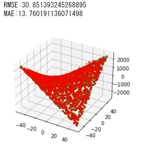
LightGBMもTree-Basedなモデルであるため決定木やランダムフォレストと同様良い結果を示した.
結果
線形回帰
和:RMSE:7.687172784612035e-15, MAE:6.2985727744546695e-15
積:RMSE:860.2557991900233, MAE:645.6874986349678
サポートベクターマシン
和:RMSE:6.291793596953627, MAE:4.97
積:RMSE:367.056421639326, MAE:290.57
決定木
和:RMSE:1.764936259472279, MAE:1.3483333333333334
積:RMSE:43.582603563042596 MAE:28.223333333333333
ランダムフォレスト
和:RMSE:0.8473663119729665, MAE:0.6351666666666667
積:RMSE:29.204948422028302, MAE:14.404766666666665
全結合ニューラルネットワーク
和:RMSE:0.14495966776685032, MAE:0.12204069801606238
積:RMSE:13.27449035031233, MAE:10.106990229040385
LightGBM
和:RMSE:0.47721846858535866, MAE:0.3211128216860885
積:RMSE:30.851393245268895, MAE:13.760191136071498
和:線形回帰が最強でしたが、他のモデルもしっかり認識しました.
積:ニューラルネットワークやTree-Basedな手法が強かったです.