pandasデータフレームからpolar(極座標)プロット

最終的にデータフレームからこんな極座標プロットを描けるようにします。
matplotlibを利用してのプロットはコードが煩雑になりやすいので、なるべくpandas.DataFrameのメソッドとして呼び出してコンパクトなコードでプロットできるようにします。

モジュールインポート

import polar

使用するコードはこれだけです。

polar.py

#!/usr/bin/env python
"""polar plot functions"""
import pandas as pd
import numpy as np
import matplotlib.pyplot as plt
import plotly.graph_objs as go
import plotly.offline
plotly.offline.init_notebook_mode(connected=False)


def _polarplot(df, **kwargs):
    """polar plot
    usage: df.polarplot()
    Same args with `df.plot()`
    """
    _df = df.copy()
    _df.index = _df.index * np.pi / 180  # Convert radian
    ax = plt.subplot(111, projection='polar')  # Polar plot
    ax = _df.plot(ax=ax, **kwargs)
    return ax


def _ipolarplot(df, layout=None, *args, **kwargs):
    """polar iplot
        usage:
            df.ipolarplot(layout=<layout>, mode=<mode>, marker=<marker>...)

        args:
            df: Data (pandas.Series or DataFrame object)
            layout: go.Layout args (dict like)
            *args, **kwargs: Scatterpolar args such as marker, mode...

        return:
            plotly.offline.iplot(data, layout)
    """
    if isinstance(df, pd.Series):  # Type Series
        data = [go.Scatterpolar(r=df, theta=df.index)]
    else:  # Type DataFrame
        data = list()
        for _data in df.columns:
            # Make polar plot data
            polar = go.Scatterpolar(
                r=df[_data], theta=df.index, name=_data, *args, **kwargs)
            data.append(polar)  # Append all columns in data
    # Use layout if designated
    fig = go.Figure(data=data) if not layout\
        else go.Figure(data=data, layout=go.Layout(layout))
    return plotly.offline.iplot(fig)


def _mirror(df, ccw=True):
    """Make a mirror copy of DataFrame with respect to the line
    usage:
        df.mirror(ccw=True)...data increase to Counter Clock Wise(ccw)
        df.mirror(ccw=False)...data increase to Clock Wise(cw)
    args: ccw(bool) default True
    return: pandas.Series or pandas.DataFrame
    """
    copy_index = df.index
    if ccw:  # data increase to Counter Clock Wise(ccw)
        mirror_df = df.append(df.iloc[-2::-1], ignore_index=True)
        new_index = np.r_[copy_index, copy_index[1:] + copy_index[-1]]
    else:  # data increase to Clock Wise(cw)
        mirror_df = df.iloc[::-1].append(df.iloc[1:], ignore_index=True)
        new_index = np.r_[copy_index[::-1], -copy_index[1:]]
    mirror_df.index = new_index  # reset index
    return mirror_df


# Use as pandas methods
for cls in (pd.DataFrame, pd.Series):
    setattr(cls, 'polarplot', _polarplot)
    setattr(cls, 'ipolarplot', _ipolarplot)
    setattr(cls, 'mirror', _mirror)

Seriesで極座標プロット

サンプルデータ

10°刻みで0°から90°までランダムな値が入ったデータを用意します。
以下では断りがない限り、indexの単位はすべて度数法に準じた"°(度)"です。

np.random.seed(6)  # ランダムステート固定
index = range(0,190,10)
sr = pd.Series(np.random.randn(len(index)), index=index); sr

0     -0.311784
10     0.729004
20     0.217821
30    -0.899092
40    -2.486781
50     0.913252
60     1.127064
70    -1.514093
80     1.639291
90    -0.429894
100    2.631281
110    0.601822
120   -0.335882
130    1.237738
140    0.111128
150    0.129151
160    0.076128
170   -0.155128
180    0.634225
dtype: float64

極座標プロット

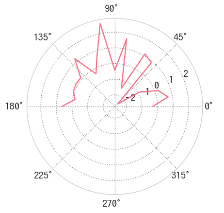
polarplot()メソッドでサンプルデータを極座標にプロットします。
polar.pyをインポートしてしまえば、pandas.Series, pandas.DataFrame型からpolarplot()メソッドが使えるようになっています。

sr.polarplot()

polarplot.py

def _polarplot(df, **kwargs):
    _df = df.copy()
    _df.index = _df.index * np.pi / 180  # Convert radian
    ax = plt.subplot(111, projection='polar')  # Polar plot
    ax = _df.plot(ax=ax, **kwargs)
    return ax

polarplot()メソッドは引数にデータフレーム(またはシリーズ)を要求して、戻り値はグラフaxです。
**kwargs引数で、df.plot()と同じ引数が使えます。

pandasのメソッドとして使えるように、ファイルの一番下でsetattr(pd.DataFrame, 'polarplot', _polarplot)としてあるので、df.polarplot()として呼び出せます。

pd.DataFrame.polarplot = _polarplotとすることと同じです。自作の関数を既存クラスのメソッドとして扱えるようにする私の常套手段です。

鏡像データを作成

mirror()メソッドで、鏡像データを作り出します。

データの中身は次に示すように360°方向に増えます。

sr.mirror()

0     -0.311784
10     0.729004
20     0.217821
30    -0.899092
40    -2.486781
50     0.913252
60     1.127064
70    -1.514093
80     1.639291
90    -0.429894
100    2.631281
110    0.601822
120   -0.335882
130    1.237738
140    0.111128
150    0.129151
160    0.076128
170   -0.155128
180    0.634225
190   -0.155128
200    0.076128
210    0.129151
220    0.111128
230    1.237738
240   -0.335882
250    0.601822
260    2.631281
270   -0.429894
280    1.639291
290   -1.514093
300    1.127064
310    0.913252
320   -2.486781
330   -0.899092
340    0.217821
350    0.729004
360   -0.311784
dtype: float64

mirror.py

def _mirror(df, ccw=True):
    copy_index = df.index
    if ccw:  # data increase to Counter Clock Wise(ccw)
        mirror_df = df.append(df.iloc[-2::-1], ignore_index=True)
        new_index = np.r_[copy_index, copy_index[1:] + copy_index[-1]]
    else:  # data increase to Clock Wise(cw)
        mirror_df = df.iloc[::-1].append(df.iloc[1:], ignore_index=True)
        new_index = np.r_[copy_index[::-1], -copy_index[1:]]
    mirror_df.index = new_index  # reset index
    return mirror_df

引数無し、またはccw=Trueでmirror()メソッドを呼ぶと、反時計回りにデータをコピーして、インデックスを振り直します。
引数ccw=Falseでmirror()メソッドを呼ぶと、時計回りにデータをコピーして、インデックスを振り直します。

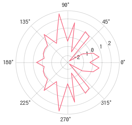
mirror化したシリーズをプロットします。

sr.mirror().polarplot()

DataFrameで極座標プロット

sin波サンプルデータ

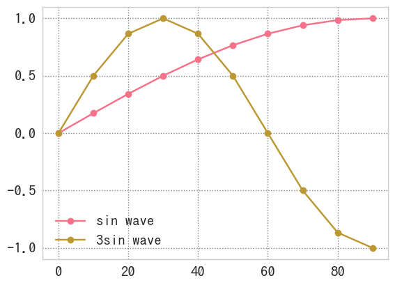
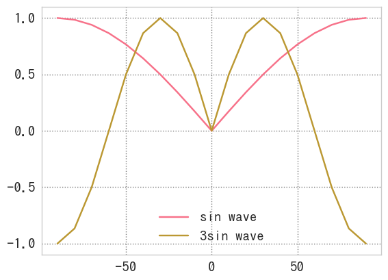
次に、DataFrame型で極座標プロットを行います。
sin波を$\pi$/2だけとったサンプルデータを作成します。

SeriesだろうがDataFrameだろうが使い方は同じです。

index = np.arange(0,100,10)
df = pd.DataFrame({'sin wave':np.sin(index*np.pi/180),
                   '3sin wave':np.sin(3*index*np.pi/180)}, index=index)
df.plot(style='o-')

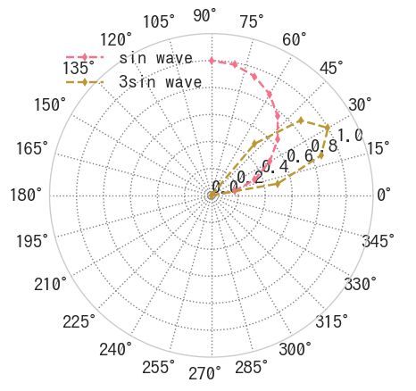
polarplotの引数指定

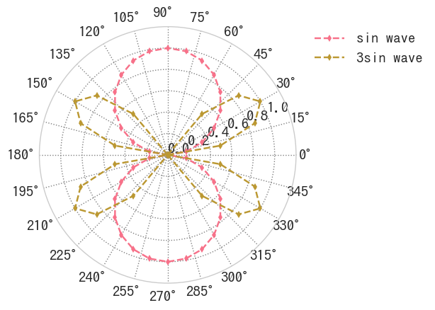
極座標プロットするためにpolarplot()メソッドを使用します。
polarplot()メソッドの引数にはdf.plot(**kwargs)として使えるほぼすべての引数が使えます。

例えば以下のようにしてstyleやmsを指定してあげると、線種を変えたり、marker sizeを変更してくれます。

df.polarplot(style='d--', ms=5,
             ylim=[0,1.2], yticks=np.arange(0,1.2,.2),
             xticks=np.arange(1,360,15)*np.pi/180)

ミラー化(CCW=反時計回り)

デフォルトでは、mirror()メソッドは反時計回りに鏡像を作成します。

df.mirror()

	sin wave	3sin wave
0	0.000000	0.000000e+00
10	0.173648	5.000000e-01
20	0.342020	8.660254e-01
30	0.500000	1.000000e+00
40	0.642788	8.660254e-01
50	0.766044	5.000000e-01
60	0.866025	1.224647e-16
70	0.939693	-5.000000e-01
80	0.984808	-8.660254e-01
90	1.000000	-1.000000e+00
100	0.984808	-8.660254e-01
110	0.939693	-5.000000e-01
120	0.866025	1.224647e-16
130	0.766044	5.000000e-01
140	0.642788	8.660254e-01
150	0.500000	1.000000e+00
160	0.342020	8.660254e-01
170	0.173648	5.000000e-01
180	0.000000	0.000000e+00

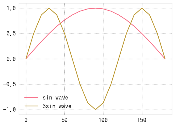
デカルト座標系にプロットするとこんな感じです。

df.mirror().plot()

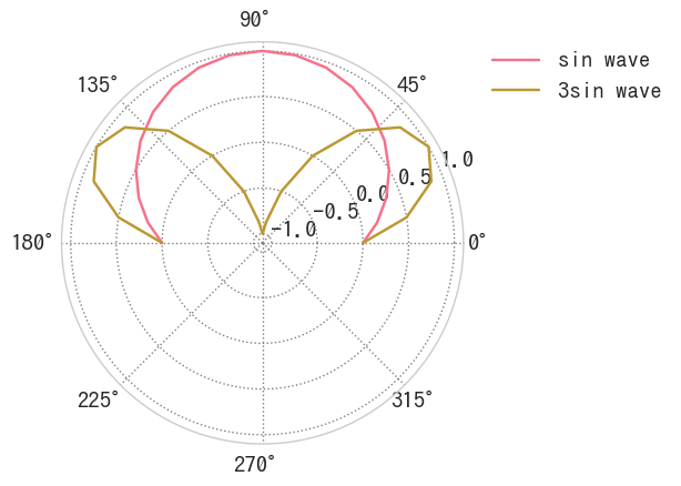
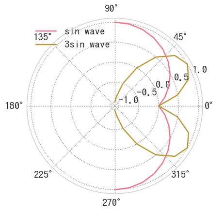
極座標プロットでは判例が間違いなくグラフの円の中に含まれて重なって見づらいので、凡例を外側に置くようにplt.legend()で凡例の位置を指定したほうが良いです。

df.mirror().polarplot()
plt.legend(bbox_to_anchor=(1.05, 1), loc=2, borderaxespad=0)  # 凡例外側

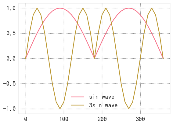
1周(360度)までデータを拡張するにはmirror()メソッドを2回続けて打って下さい。

df.mirror().mirror()

	sin wave	3sin wave
0	0.000000	0.000000e+00
10	0.173648	5.000000e-01
20	0.342020	8.660254e-01
30	0.500000	1.000000e+00
40	0.642788	8.660254e-01
50	0.766044	5.000000e-01
60	0.866025	1.224647e-16
70	0.939693	-5.000000e-01
80	0.984808	-8.660254e-01
90	1.000000	-1.000000e+00
100	0.984808	-8.660254e-01
110	0.939693	-5.000000e-01
120	0.866025	1.224647e-16
130	0.766044	5.000000e-01
140	0.642788	8.660254e-01
150	0.500000	1.000000e+00
160	0.342020	8.660254e-01
170	0.173648	5.000000e-01
180	0.000000	0.000000e+00
190	0.173648	5.000000e-01
200	0.342020	8.660254e-01
210	0.500000	1.000000e+00
220	0.642788	8.660254e-01
230	0.766044	5.000000e-01
240	0.866025	1.224647e-16
250	0.939693	-5.000000e-01
260	0.984808	-8.660254e-01
270	1.000000	-1.000000e+00
280	0.984808	-8.660254e-01
290	0.939693	-5.000000e-01
300	0.866025	1.224647e-16
310	0.766044	5.000000e-01
320	0.642788	8.660254e-01
330	0.500000	1.000000e+00
340	0.342020	8.660254e-01
350	0.173648	5.000000e-01
360	0.000000	0.000000e+00

df.mirror().mirror().plot()

df.mirror().mirror().polarplot(df.polarplot(style='d--', ms=5,
                               ylim=[0,1.2], yticks=np.arange(0,1.2,.2),
                               xticks=np.arange(1,360,15)*np.pi/180))
plt.legend(bbox_to_anchor=(1.05, 1), loc=2, borderaxespad=0)  # 凡例外側

ミラー化(CW=時計回り)

mirror()メソッドの引数はcw(Counter Cloce Wise 反時計回り)のみで、デフォルトはTrueです。
mirror(False)のようにしてメソッドの引数を指定するとcw(Cloce Wise 時計回り)でデータを作成します。

df.mirror(False)

	sin wave	3sin wave
90	1.000000	-1.000000e+00
80	0.984808	-8.660254e-01
70	0.939693	-5.000000e-01
60	0.866025	1.224647e-16
50	0.766044	5.000000e-01
40	0.642788	8.660254e-01
30	0.500000	1.000000e+00
20	0.342020	8.660254e-01
10	0.173648	5.000000e-01
0	0.000000	0.000000e+00
-10	0.173648	5.000000e-01
-20	0.342020	8.660254e-01
-30	0.500000	1.000000e+00
-40	0.642788	8.660254e-01
-50	0.766044	5.000000e-01
-60	0.866025	1.224647e-16
-70	0.939693	-5.000000e-01
-80	0.984808	-8.660254e-01
-90	1.000000	-1.000000e+00

df.mirror(False).plot()

df.mirror(False).polarplot()

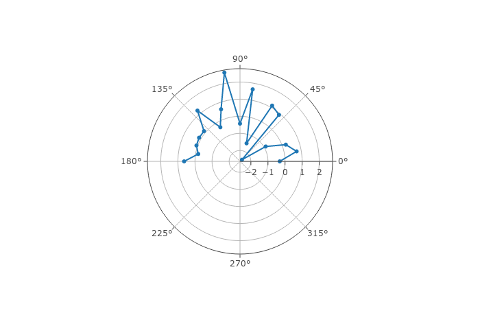
動的プロット

Polar Charts in Pythonを参考にplotlyを利用してインタラクティブな極座標プロットを描いてみます。

まずはplotlyのインポートとオフラインモードの有効化

import plotly.graph_objs as go
import plotly.offline
plotly.offline.init_notebook_mode(connected=False)

データをリスト型にしてgo.Figure()クラスの引数とします。

data = [
    go.Scatterpolar(
        r = df['sin wave'],
        theta = df.index,
    ),
    go.Scatterpolar(
        r = df['3sin wave'],
        theta = df.index,
    )
]

fig = go.Figure(data=data)
plotly.offline.iplot(fig)

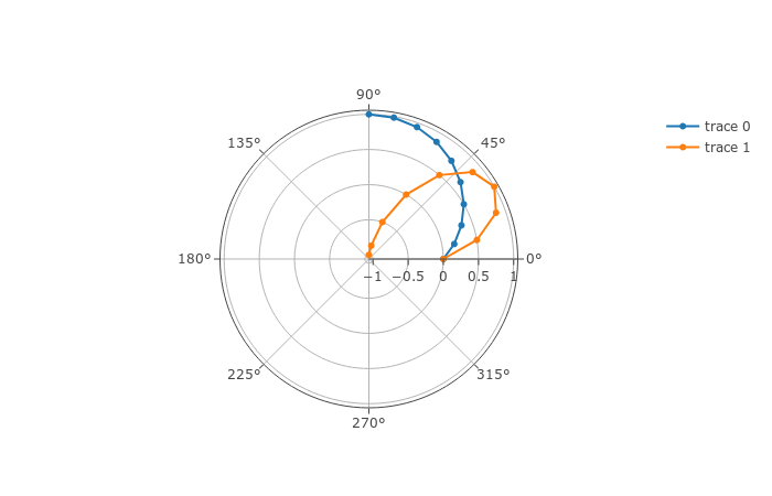
これを参考にpolarplot()をまねてipolarplot()を作成しました。

_ipolarplot.py

def _ipolarplot(df, layout=None, *args, **kwargs):
    if isinstance(df, pd.Series):  # Type Series
        data = [go.Scatterpolar(r=df, theta=df.index)]
    else:  # Type DataFrame
        data = list()
        for _data in df.columns:
            # Make polar plot data
            polar = go.Scatterpolar(
                r=df[_data], theta=df.index, name=_data, *args, **kwargs)
            data.append(polar)  # Append all columns in data
    # Use layout if designated
    fig = go.Figure(data=data) if not layout\
        else go.Figure(data=data, layout=go.Layout(layout))
    return plotly.offline.iplot(fig)

for cls in (pd.DataFrame, pd.Series):
    setattr(cls, 'ipolarplot', _ipolarplot)

sr.ipolarplot()

df.ipolarplot()

**kwargsとして、go.Scatter()に渡す引数と同じものが使えます。
レイアウトは辞書型として内部的にgo.Layout()に渡しています。

df.mirror().ipolarplot(mode='markers', layout=dict(title='sin & 3sin', showlegend=False))

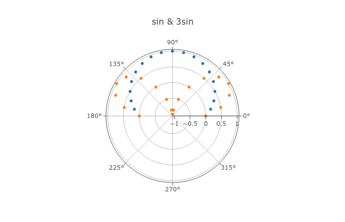
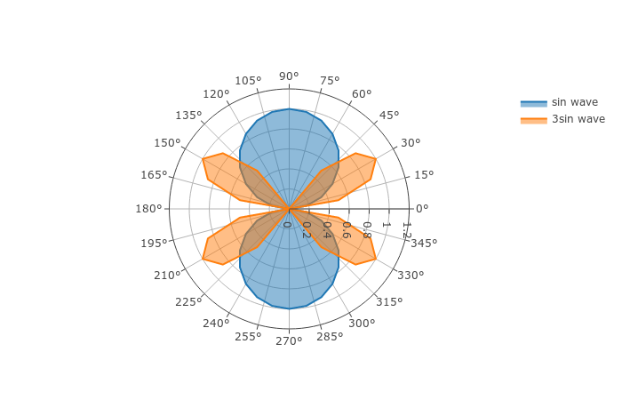
塗りつぶしやレンジ、ティックスの幅を変えることもできますが、plotlyの指定の仕方はやや複雑です。

plotly polarchartの複雑な設定は先にも挙げたPolar Charts in Pythonを参考にしました。

df.mirror().mirror().ipolarplot(fill='toself',
                                layout=dict(
                                    polar=dict(
                                        radialaxis = dict(
                                                        visible=True,
                                                        range=[0,1.2],
                                                    ),
                                        angularaxis = dict(
                                                        dtick=15
                                                        )
                                            )
                                       )
                                )

まとめ

polar.pyを使用して次のことができました。

• polarplot()メソッドによりデータフレームから極座標プロットをメソッドとして扱えるようになりました。
• mirror()メソッドにより線対称にデータを増やすことが可能になりました。
• plotlyを利用したipolarplot()メソッドを使用して、ズームイン、ズームアウト、数値をインタラクティブに表示可能なプロットを描けました。

コードとjupyter notebookはgithubにあげました。
u1and0/polarplot