概要
物理シミュレーションの第一歩ということで、単振り子(pendulum)および二重振り子(double pendulum)をつくってみました.
二重振り子については,軌跡付きでつくってみました.
動作環境
- Windows10(64bit)
- Python 3.7.2
単振り子の理論
まずは,単振り子の運動方程式を導きます.
直交座標系の運動方程式を立ててから,角度のみの運動方程式に変形してもいいのですが,
ラグランジアンを使って導いた方がラクでしょう.
振り子が鉛直方向となす角を$\theta$とすると,
運動エネルギー
K=\frac{1}{2}m\dot{x}^2=\frac{1}{2}m{(l\dot{\theta})}^2
ポテンシャル
U=mglcos\theta
ゆえにラグランジアンは
\begin{align}
L & = K - U\\
& = \frac{1}{2}m{(l\dot{\theta})}^2 - mglcos\theta
\end{align}
オイラーラグランジュ方程式に代入して
\begin{align}
\frac{d}{dt}(ml^2(\dot{\theta}^2) + mglsin\theta)  = 0\\
ml^2\ddot{\theta}  = -mglsin\theta\\
\ddot{\theta}  = -\frac{g}{l}sin\theta
\end{align}
となり,$\theta$に関する二階の微分方程式を得る.
Pythonで解くときには,微分方程式は一階の微分方程式にする必要があるが,
一般に$n$階の微分方程式は$n$次の連立微分方程式に変形することができる.
今の場合,以下のように$\theta$に関する二階微分方程式が$\theta$と$\omega$に関する連立一階微分方程式に変形ができる.
\begin{cases}
\dot{\theta} & = \omega\\
\dot{\omega} & = -\frac{g}{l}sin\theta
\end{cases}
微分方程式を解く方法
Pythonで微分方程式を解くためには,scipy.integrateの中のodeintやodeがありますし,
実際この関数を使ったコードはネット上にも多く見られました.
しかし,odeintの公式ドキュメントを見てみると,微分方程式を解くための新しい関数として
scipy.integrate.solve_ivpが推奨されています.
ということで,今回は,solve_ivp()を使っていこうと思います.
使い方を具体例を使って説明していきます。
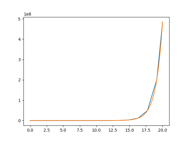
- 例1
\frac{dy}{dt}=y\\
y(0)=1
解:$y = exp(t)$
def func (t, y):
    dydt = y
    return dydt

sol = scipy.integrate.solve_ivp(func, [0,20], [1])
t1 = sol.t
y1 = sol.y.T

t2 = np.linspace(0, 20, 100)
plt.plot(t1, y1)
plt.plot(t2, np.exp(t2))
plt.show()
solve_ivp()の第1引数は微分値を返す関数です.つまり,以下の方程式で言う右辺を返り値に持つ関数です.
\frac{dy}{dt} = f(t, y)
solve_ivp()第2引数は時間を,第3引数は初期値を取ります.今回は,$t=0$から$t=20$までとしました.
時間の刻み幅自動で設定されます.これはodeintなどとの違いの一つです.
もし,刻み幅を指定したい場合は例2のようにt_evalキーワードを追加します.
実行結果は以下のようになります.
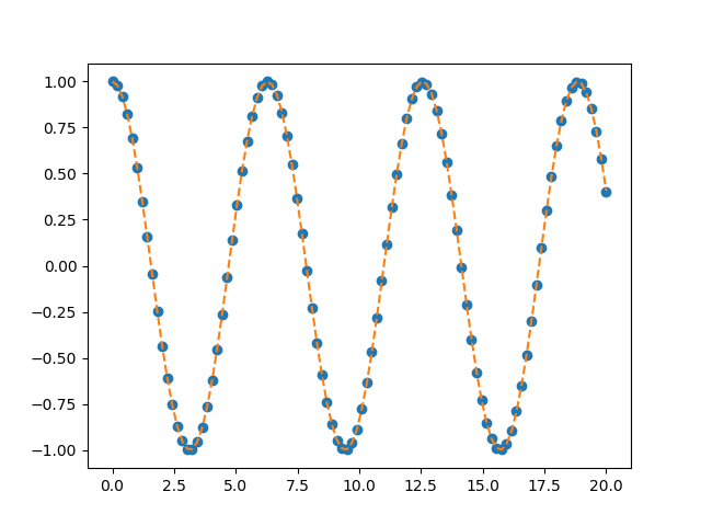
- 例2
\frac{d^2y}{dt^2}=-y\\
y(0)=1\\
\frac{dy}{dt}(0)=0\\
解:$y = cos(t)$
例2は2階の微分方程式です.関数funcの中身は上記のようになります.
考え方としては,
y = y_0\\
\frac{dy}{dt} = y_1
として,以下の連立1階微分方程式に帰着させます.
\frac{d}{dt}y_0 = y_1\\
\frac{d}{dt}y_1 = -y_0
def func (t, y):
    dydt = np.zeros_like(y)
    dydt[0] = y[1]
    dydt[1] = -y[0]
    return dydt

t_span=[0,20]
y0 = [0,1]
t = np.linspace(t_span[0], t_span[1], 100)
sol = scipy.integrate.solve_ivp(func, t_span, y0, t_eval=t)
t1 = sol.t
y1 = sol.y[1,:]

t2 = np.linspace(0, 20, 100)
plt.plot(t1, y1, 'o')
plt.plot(t2, np.cos(t2), '--')
plt.show()
実行結果は以下のようになります.
単振り子の実装
それでは,単振り子のシミュレーションを行うプログラムを実装してみましょう!
from numpy import sin, cos
from scipy.integrate import solve_ivp
from matplotlib.animation import FuncAnimation
import matplotlib.pyplot as plt
import numpy as np

G = 9.8                                 # 重力加速度 [m/s^2]
L = 1.0                                 # 振り子の長さ [m]

# 運動方程式
def derivs(t, state):
    dydt = np.zeros_like(state)
    dydt[0] = state[1]
    dydt[1] = -(G/L)*sin(state[0])
    return dydt

t_span = [0,20]                         # 観測時間 [s]
dt = 0.05                               # 間隔 [s]
t = np.arange(t_span[0], t_span[1], dt)
th1 = 30.0                              # 初期角度 [deg]
w1 = 0.0                                # 初期角速度 [deg/s]
state = np.radians([th1, w1])           # 初期状態

sol = solve_ivp(derivs, t_span, state, t_eval=t)
theta = sol.y[0,:]
print(np.shape(sol.y))

x = L * sin(theta)       # x = Lsin(theta)
y = -L * cos(theta)      # y = -Lcos(theta)

fig, ax = plt.subplots()

line, = ax.plot([], [], 'o-', linewidth=2) # このlineに次々と座標を代入して描画

def animate(i):
    thisx = [0, x[i]]
    thisy = [0, y[i]]

    line.set_data(thisx, thisy)
    return line,

ani = FuncAnimation(fig, animate, frames=np.arange(0, len(t)), interval=25, blit=True)

ax.set_xlim(-L,L)
ax.set_ylim(-L,L)
ax.set_aspect('equal')
ax.grid()
plt.show()

# ani.save('pendulum.gif', writer='pillow', fps=15)
解説
- ライブラリのインポート
まずは,必要なライブラリをインポートします.
from numpy import sin, cos
from scipy.integrate import solve_ivp
from matplotlib.animation import FuncAnimation
import matplotlib.pyplot as plt
import numpy as np
- 運動方程式の記述
続いて運動方程式を記述する関数を定義します.重力加速度はG,振り子の長さはLとしています.
def derivs(t, state):
    dydt = np.zeros_like(state)
    dydt[0] = state[1]
    dydt[1] = -(G/L)*sin(state[0])
    return dydt
- 初期条件の記述
運動方程式の初期条件を与えます.2階微分方程式なので自由度は2ですね.
th1 = 30.0
w1 = 0.0
state = np.radians([th1, w1])
- 運動方程式を解く
運動方程式の数値解を求めます.
yは(2,len(t))型の二次元配列なので,今は,1行目の角度$\theta$のみを取得します.
2行目の角速度$\omega$は今回は必要ないです.
sol = solve_ivp(derivs, t_span, state, t_eval=t)
theta = sol.y[0,:]
- 直交座標系に変換
求まった$\theta$から直交座標系$(x,y)$に変換します.これでデータは得られました.
あとは,これをプロットするだけです.
x = L * sin(theta)
y = -L * cos(theta)
- 逐次描画していく関数の定義
順次描画していくための関数を定義します.1行目のlineに次々と座標を代入して描画をしていきます.
linewidth=2はlw=2と省略することもできます.'o-'は端点と線分を表します.
line, = ax.plot([], [], 'o-', linewidth=2)

def animate(i):
    x = [0, x[i]]
    y = [0, y[i]]

    line.set_data(x, y)
    return line,
- アニメーションの関数
最後にアニメーションを実行します.
blitキーワードやintervalキーワードはアニメーションが滑らかになるように設定しています.なくても動きます.
あとは,レイアウトなどを整え,プロットすれば終わりです.
ani = FuncAnimation(fig, animate, frames=np.arange(0, len(t)), interval=25, blit=True)
実行結果
二重振り子
では,単振り子でアニメーションの方法はマスターできたと思うので,二重振り子をシミュレーションしてみましょう.
カオスが見れて面白いです!
さらに,単振り子のレベルアップということで軌跡も描画しちゃいましょう.
二重振り子の理論
二重振り子の運動方程式も単振り子同様ラグランジアンを求めて,オイラーラグランジュ方程式に代入すれば求まります.
詳しくは,こちら!
https://youtu.be/llCSRuRqnEw
\begin{cases}
(x_1, y_1) = (l_1sin\theta_1, l_1cos\theta_1)\\
(x_2, y_2) = (l_1sin\theta_1 + l_2sin\theta_2, l_1cos\theta_1 + l_2cos\theta_2)
\end{cases}\\
\begin{cases}
(\dot{x_1}, \dot{y_1}) = (l_1\dot{\theta_1}cos\theta_1, -l_1\dot{\theta_1}sin\theta_1)\\
(\dot{x_2}, \dot{y_2}) = (l_1\dot{\theta_1}cos\theta_1 + l_2\dot{\theta_2}cos\theta_2, -l_1\dot{\theta_1}sin\theta_1 - l_2\dot{\theta_2}sin\theta_2)
\end{cases}
運動エネルギー
\begin{align}
K & = \frac{1}{2}\Bigl((\dot{x_1})^2 + (\dot{y_1})^2\Bigr) + \frac{1}{2}\Bigl((\dot{x_2})^2 + (\dot{y_2})^2\Bigr)\\
& = \frac{1}{2}m_1(l_1\dot{\theta_1})^2 + \frac{1}{2}m_2\Bigl((l_1\dot{\theta_1})^2 + (l_2\dot{\theta_2})^2 + 2l_1l_2\dot{\theta_1}\dot{\theta_2}cos{(\theta_1-\theta_2)} \Bigr)\\
& = \frac{1}{2}(m_1+m_2)(l_1\dot{\theta_1})^2 + \frac{1}{2}m_2(l_2\dot{\theta_2})^2 + m_2l_1l_2\dot{\theta_1}\dot{\theta_2}cos({\theta_1-\theta_2})
\end{align}
ポテンシャル
\begin{align}
U & = -m_1gy_1 - m_2gy_2\\
& = -m_1gl_1cos\theta_1-m_2g(l_1cos\theta_1+l_2cos\theta_2)\\
& = -(m_1+m_2)gl_1cos\theta_1 - m_2gl_2cos\theta_2
\end{align}
ラグランジアン
\begin{align}
L & = K - U\\
& = \frac{1}{2}(m_1+m_2)(l_1\dot{\theta_1})^2 + \frac{1}{2}m_2(l_2\dot{\theta_2})^2 + m_2l_1l_2\dot{\theta_1}\dot{\theta_2}cos({\theta_1-\theta_2})\\
&  + (m_1+m_2)gl_1cos\theta_1 + m_2gl_2cos\theta_2\\
\end{align}
ここで、
\begin{cases}
\frac{\partial L}{\partial \theta_1} = -m_2l_1l_2\dot{\theta_1}\dot{\theta_2}sin(\theta_1-\theta_2) + (m_1+m_2)gl_1sin\theta_1 \\
\frac{\partial L}{\partial \dot{\theta_1}} = (m_1+m_2)l_1^2\dot{\theta_1} + m_2l_1l_2\dot{\theta_2}cos(\theta_1-\theta_2) \\
\frac{\partial L}{\partial \theta_2} = m_2l_1l_2\dot{\theta_1}\dot{\theta_2}sin(\theta_1-\theta_2) \\
\frac{\partial L}{\partial \dot{\theta_2}} = m_2l_2^2\dot{\theta_2} + m_2l_1l_2\dot{\theta_1}cos(\theta_1-\theta_2)
\end{cases}
時間で微分して、
\begin{cases}
\frac{d}{dt}\frac{\partial L}{\partial \dot{\theta_1}} = (m_1+m_2)l_1^2\ddot{\theta_1} + m_2l_1l_2\Bigl(\ddot{\theta_2}cos(\theta_1-\theta_2) - \dot{\theta_1}\dot{\theta_2}sin(\theta_1-\theta_2) + (\dot{\theta_2})^2sin(\theta_1-\theta_2)  \Bigr) \\
\frac{d}{dt}\frac{\partial L}{\partial \dot{\theta_2}} = m_2l_2^2\ddot{\theta_2} + m_2l_1l_2\Bigl(\ddot{\theta_1}cos(\theta_1-\theta_2) -(\dot{\theta_1})^2sin(\theta_1-\theta_2) + \dot{\theta_1}\dot{\theta_2}sin(\theta_1-\theta_2) \Bigr)
\end{cases}
オイラーラグランジュ方程式に代入して、以下の運動方程式を得る。
\begin{cases}
(m_1+m_2)l_1^2\ddot{\theta_1}+m_2l_1l_2\ddot{\theta_2}cos(\theta_1-\theta_2)+m_2l_1l_2(\dot{\theta_2})^2sin(\theta_1-\theta_2)+(m_1+m_2)l_1gsin\theta_1 = 0 \\
m_2l_1l_2\ddot{\theta_1}cos(\theta_1-\theta_2)+m_2l_2^2\ddot{\theta_2}-m_2l_1l_2(\dot{\theta_1})^2sin(\theta_1-\theta_2)+m_2gl_2sin\theta_2 = 0
\end{cases}
上式は$l_1$で,下式は$m_2l_2$で割って,
$\varDelta=\theta_2-\theta_1$, $\dot{\theta_1}=\omega_1$, $\dot{\theta_2}=\omega_2$として整理すると
\begin{pmatrix}
(m_1+m_2)l_1 & m_2l_2cos\varDelta \\
l_1cos\varDelta & l_2
\end{pmatrix}

\begin{pmatrix}
\dot{\omega_1}\\
\dot{\omega_2}
\end{pmatrix}

=

\begin{pmatrix}
m_2l_2(\omega_2)^2sin\varDelta - (m_1+m_2)gsin{\theta_1}\\
l_1(\omega_1)^2 sin\varDelta -gsin{\theta_2}
\end{pmatrix}
$\dot{\omega_1}, \dot{\omega_2}$について解くと,
\dot{\omega_1} = \frac{
\begin{vmatrix}
m_2l_2(\omega_2)^2sin\varDelta-(m_1+m_2)gsin{\theta_1} & m_2l_2cos\varDelta \\
l_1(\omega_1)^2sin\varDelta-gsin{\theta_2} & l_2
\end{vmatrix}}{
\begin{vmatrix}
(m_1+m_2)l_1 & m_2l_2cos\varDelta \\
l_1cos\varDelta & l_2 \\
\end{vmatrix}} \\
\dot{\omega_2} = \frac{
\begin{vmatrix}
(m_1+m_2)l_1 & m_2l_2(\omega_2)^2sin\varDelta-(m_1+m_2)gsin{\theta_1} \\
l_1cos\varDelta & l_1(\omega_1)^2sin\varDelta-gsin{\theta_2}
\end{vmatrix}}{
\begin{vmatrix}
(m_1+m_2)l_1 & m_2l_2cos\varDelta \\
l_1cos\varDelta & l_2
\end{vmatrix}}
より
\begin{cases}
\frac{d\theta_1}{dt} = \omega_1\\
\frac{d\omega_1}{dt} = \frac{m_2l_1\omega_1^2sin\varDelta cos\varDelta + m_2gsin\theta_2cos\varDelta + m_2l_2\omega_2^2sin\varDelta -(m_1+m_2)gsin\theta_1}{(m_1+m_2)l_1-m_2l_1cos^2{\varDelta}}\\
\frac{d\theta_2}{dt} = \omega_2\\
\frac{d\omega_2}{dt} = \frac{-m_2l_2\omega_2^2sin\varDelta cos\varDelta + (m_1+m_2)gsin\theta_1cos\varDelta -(m_1+m_2)l_1\omega_1^2sin\varDelta -(m_1+m_2)gsin\theta_2}{(m_1+m_2)l_1-m_2l_1cos^2{\varDelta}}
\end{cases}
となり、一階連立微分方程式に帰着させることができた.
二重振り子の実装
それでは,二重振り子のシミュレーションを行うプログラムを実装しています.
matplotlibの公式ドキュメントに二重振り子のシミュレーションプログラムがあるのでそちらを参考にしました.
from numpy import sin, cos
from scipy.integrate import solve_ivp
from matplotlib.animation import FuncAnimation
import numpy as np
import matplotlib.pyplot as plt


G = 9.8     # 重力加速度 [m/s^2]
L1 = 1.0    # 単振り子1の長さ [m]
L2 = 1.0    # 単振り子2の長さ [m]
M1 = 1.0    # おもり1の質量 [kg]
M2 = 1.0    # おもり2の質量 [kg]

# 運動方程式
def derivs(t, state):

    dydx = np.zeros_like(state)
    dydx[0] = state[1]

    delta = state[2] - state[0]
    den1 = (M1+M2) * L1 - M2 * L1 * cos(delta) * cos(delta)
    dydx[1] = ((M2 * L1 * state[1] * state[1] * sin(delta) * cos(delta)
                + M2 * G * sin(state[2]) * cos(delta)
                + M2 * L2 * state[3] * state[3] * sin(delta)
                - (M1+M2) * G * sin(state[0]))
               / den1)

    dydx[2] = state[3]

    den2 = (L2/L1) * den1
    dydx[3] = ((- M2 * L2 * state[3] * state[3] * sin(delta) * cos(delta)
                + (M1+M2) * G * sin(state[0]) * cos(delta)
                - (M1+M2) * L1 * state[1] * state[1] * sin(delta)
                - (M1+M2) * G * sin(state[2]))
               / den2)

    return dydx

# 時間生成
t_span = [0,20]
dt = 0.05
t = np.arange(t_span[0], t_span[1], dt)

# 初期条件
th1 = 120.0
w1 = 0.0
th2 = -10.0
w2 = 0.0
state = np.radians([th1, w1, th2, w2])

# 運動方程式を解く
sol = solve_ivp(derivs, t_span, state, t_eval=t)
y = sol.y

# ジェネレータ
def gen():
    for tt, th1, th2 in zip(t,y[0,:], y[2,:]):
        x1 = L1*sin(th1)
        y1 = -L1*cos(th1)
        x2 = L2*sin(th2) + x1
        y2 = -L2*cos(th2) + y1
        yield tt, x1, y1, x2, y2

fig, ax = plt.subplots()
ax.set_xlim(-(L1+L2), L1+L2)
ax.set_ylim(-(L1+L2), L1+L2)
ax.set_aspect('equal')
ax.grid()

locus, = ax.plot([], [], 'r-', linewidth=2)
line, = ax.plot([], [], 'o-', linewidth=2)
time_template = 'time = %.1fs'
time_text = ax.text(0.05, 0.9, '', transform=ax.transAxes)

xlocus, ylocus = [], []
def animate(data):
    t, x1, y1, x2, y2 = data
    xlocus.append(x2)
    ylocus.append(y2)

    locus.set_data(xlocus, ylocus)
    line.set_data([0, x1, x2], [0, y1, y2])
    time_text.set_text(time_template % (t))

ani = FuncAnimation(fig, animate, gen, interval=50, repeat=True)

plt.show()

# ani.save('double_pendulum.gif', writer='pillow', fps=15)
解説
- 運動方程式の記述
def derivs(t, state):

    dydx = np.zeros_like(state)
    dydx[0] = state[1]

    delta = state[2] - state[0]
    den1 = (M1+M2) * L1 - M2 * L1 * cos(delta) * cos(delta)
    dydx[1] = ((M2 * L1 * state[1] * state[1] * sin(delta) * cos(delta)
                + M2 * G * sin(state[2]) * cos(delta)
                + M2 * L2 * state[3] * state[3] * sin(delta)
                - (M1+M2) * G * sin(state[0]))
               / den1)

    dydx[2] = state[3]

    den2 = (L2/L1) * den1
    dydx[3] = ((- M2 * L2 * state[3] * state[3] * sin(delta) * cos(delta)
                + (M1+M2) * G * sin(state[0]) * cos(delta)
                - (M1+M2) * L1 * state[1] * state[1] * sin(delta)
                - (M1+M2) * G * sin(state[2]))
               / den2)

    return dydx
- 初期条件の記述
th1 = 100.0
w1 = 0.0
th2 = -10.0
w2 = 0.0
state = np.radians([th1, w1, th2, w2])
- 運動方程式を解く
sol = solve_ivp(derivs, t_span, state, t_eval=t)
y = sol.y
- ジェネレータ関数の定義
これは単振り子と少し異なります。軌跡を描くためにジェネレータを定義します。
ジェネレータはreturnではなくyield文で返します.
また,zip()関数を使うことで,並列的に反復処理を行えます.
def gen():
    for tt, th1, th2 in zip(t,y[0,:], y[2,:]):
        x1 = L1*sin(th1)
        y1 = -L1*cos(th1)
        x2 = L2*sin(th2) + x1
        y2 = -L2*cos(th2) + y1
        yield tt, x1, y1, x2, y2
- アニメーション関数の定義
locusにどんどん値を追加していくことで,軌跡を描画します.
また今回はタイマーもついています.
locus, = ax.plot([], [], 'r-', linewidth=2)
line, = ax.plot([], [], 'o-', linewidth=2)
time_template = 'time = %.1fs'
time_text = ax.text(0.05, 0.9, '', transform=ax.transAxes)

xlocus, ylocus = [], []
def animate(data):
    t, x1, y1, x2, y2 = data
    xlocus.append(x2)
    ylocus.append(y2)

    locus.set_data(xlocus, ylocus)
    line.set_data([0, x1, x2], [0, y1, y2])
    time_text.set_text(time_template % (t))
- アニメーションの実行
ani = FuncAnimation(fig, animate, gen, interval=50, repeat=False)
実行結果

まとめ
いかがだったでしょうか?今回は物理シミュレーションとして,単振り子と二重振り子を扱ってみました.
二重振り子のカオスが見れたときは興奮しますよね.
今回のコードに関して改善点などありましたらコメントいただけると助かります.