ニューラルネットワークの予測の不確実性（Monte Carlo dropout・実装編）

はじめに

ニューラルネットワークの予測の不確実性を算出する手法を検証します。
Jupyter Notebookは下記にあります。

概要

• 連続値を予測する回帰のためのニューラルネットワークを構築
• Monte Carlo dropoutで予測の不確実性を算出

Monte Carlo dropout

学習時は通常通りdropoutを適用して学習を行い、推論時にもdropoutを適用して、n個のパラメータ${\theta_1, \cdots, \theta_n}$をサンプリングし、事後分布の期待値と分散を計算します。

$$
\mu(y) = \frac{1}{n}\sum_{i=1}^n f(x;\theta_i)
$$
$$
{\rm Var}(y) = \sigma^2 + \frac{1}{n}\sum_{i=1}^n f(x;\theta_i)^T f(x;\theta_i) - \mu(y)^T \mu(y)
$$

手法の概要は下記記事を参照してください。

実装

1. ライブラリのインポート

必要なライブラリをインポートします。

import sys
import os

import matplotlib.pyplot as plt
import numpy as np

import torch
import torch.nn as nn
import torch.nn.functional as F

2. 実行環境の確認

使用するライブラリのバージョンや、GPU環境を確認します。
Google Colaboratoryで実行した際の例になります。

print('Python:', sys.version)
print('PyTorch:', torch.__version__)
!nvidia-smi

実行結果

Python: 3.10.12 (main, Jun 11 2023, 05:26:28) [GCC 11.4.0]
PyTorch: 2.0.1+cu118
Sat Sep  2 06:13:25 2023       
+-----------------------------------------------------------------------------+
| NVIDIA-SMI 525.105.17   Driver Version: 525.105.17   CUDA Version: 12.0     |
|-------------------------------+----------------------+----------------------+
| GPU  Name        Persistence-M| Bus-Id        Disp.A | Volatile Uncorr. ECC |
| Fan  Temp  Perf  Pwr:Usage/Cap|         Memory-Usage | GPU-Util  Compute M. |
|                               |                      |               MIG M. |
|===============================+======================+======================|
|   0  Tesla T4            Off  | 00000000:00:04.0 Off |                    0 |
| N/A   37C    P8     9W /  70W |      0MiB / 15360MiB |      0%      Default |
|                               |                      |                  N/A |
+-------------------------------+----------------------+----------------------+
                                                                               
+-----------------------------------------------------------------------------+
| Processes:                                                                  |
|  GPU   GI   CI        PID   Type   Process name                  GPU Memory |
|        ID   ID                                                   Usage      |
|=============================================================================|
|  No running processes found                                                 |
+-----------------------------------------------------------------------------+

3. データセットの作成

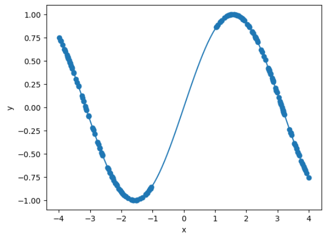
sinカーブに従うデータを作成します。
ただし、学習には[-1,1]の範囲のデータは使用しません。

def make_dataset(seed, plot=0, batch_size=64):
    np.random.seed(seed)

    x_true = np.linspace(-4, 4, 100)
    y_true = np.sin(x_true)

    x = np.concatenate([np.random.uniform(-4, -1, 100), np.random.uniform(1, 4, 100)])
    y = np.sin(x)

    # データをPyTorchのテンソルに変換
    x = torch.from_numpy(x).float().view(-1, 1)
    y = torch.from_numpy(y).float().view(-1, 1)
    x_true = torch.from_numpy(x_true).float().view(-1, 1)

    # グラフを描画
    if plot == 1:
        plt.plot(x_true, y_true)
        plt.scatter(x, y)
        plt.xlabel('x')
        plt.ylabel('y')
        plt.show()

    dataset = torch.utils.data.TensorDataset(x, y)
    data_loader = torch.utils.data.DataLoader(dataset, batch_size=batch_size, shuffle=True)
    return data_loader

_ = make_dataset(0, plot=1)

ニューラルネットワークの定義

今回は4層の全結合ニューラルネットワークを用います。

class Net(nn.Module):
    def __init__(self):
        super(Net, self).__init__()
        self.fc1 = nn.Linear(1, 1000)
        self.dropout1 = nn.Dropout(p=0.5)
        self.fc2 = nn.Linear(1000, 1000)
        self.dropout2 = nn.Dropout(p=0.5)
        self.fc3 = nn.Linear(1000, 1000)
        self.dropout3 = nn.Dropout(p=0.5)
        self.fc4 = nn.Linear(1000, 1)


    def forward(self, x):
        x = F.relu(self.fc1(x))
        x = self.dropout1(x)
        x = F.relu(self.fc2(x))
        x = self.dropout2(x)
        x = F.relu(self.fc3(x))
        x = self.dropout3(x)
        x = self.fc4(x)
        return x

4. 学習

dropoutを適用したニューラルネットワークの学習を通常通り行います。

batch_size=64
data_loader = make_dataset(0, batch_size=batch_size)

device = "cuda" if torch.cuda.is_available() else "mps" if torch.backends.mps.is_available() else "cpu"

model = Net()
model = model.to(device)
criterion = nn.MSELoss()
optimizer = torch.optim.Adam(model.parameters(), lr=1e-3, weight_decay=1e-4)


# 学習
model.train()
num_epochs = 1000
for epoch in range(num_epochs):
    for inputs, targets in data_loader:
        inputs = inputs.to(device)
        targets = targets.to(device)

        # 順伝播と損失の計算
        y_pred = model(inputs)
        loss = criterion(y_pred, targets)

        # 勾配の初期化と逆伝播
        optimizer.zero_grad()
        loss.backward()

        # パラメータの更新
        optimizer.step()

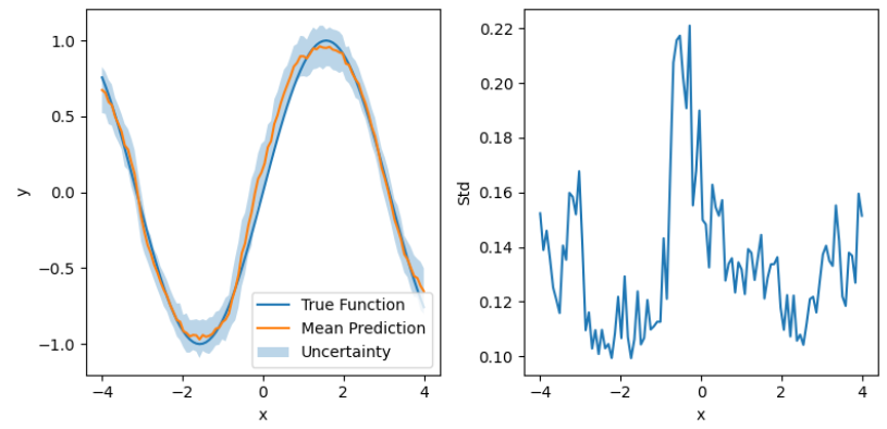
5. 予測

予測の平均と標準偏差を描画します。

x_true = np.linspace(-4, 4, 100)
y_true = np.sin(x_true)
x_true = torch.from_numpy(x_true).float().view(-1, 1)

model.train()
x_true = x_true.to(device)
y_preds = []
for _ in range(100):
    with torch.no_grad():
        y_pred = model(x_true)
    y_preds.append(y_pred.to('cpu').detach().numpy())

x_true = x_true.to('cpu')
y_preds = np.array(y_preds)
y_mean = np.mean(y_preds, axis=0)
y_std = np.std(y_preds, axis=0)


# グラフの描画
plt.figure(figsize=(8,4))

plt.subplot(121)
plt.plot(x_true, y_true, label='True Function')
plt.plot(x_true, y_mean, label='Mean Prediction')
plt.fill_between(x_true.flatten(), y_mean.flatten() - y_std.flatten(), y_mean.flatten() + y_std.flatten(), alpha=0.3, label='Uncertainty')
plt.xlabel('x')
plt.ylabel('y')
plt.legend()


plt.subplot(122)
plt.plot(x_true, y_std)
plt.xlabel('x')
plt.ylabel('Std')

plt.tight_layout()
plt.show()

plt.show()

おわりに

今回の結果

予測の不確実性は、x最小値および最大値付近とデータが含まれない[-1,1]の範囲で大きくなっています。
データ数が少なく、予測が不確実と考えられる領域と、予測の標準偏差が大きい領域が一致しているため、想定通り予測の不確実性が算出できていると考えられます。

次にやること

予測の不確実性を算出する他の手法も検証したいと思います。

参考資料

• Y. Gal and Z. Ghahramani, Dropout as a bayesian approximation: Representing model uncertainty in deep learning, ICML, 2016.
• PyTorch Quickstart
  https://pytorch.org/tutorials/beginner/basics/quickstart_tutorial.html