はじめに
国土交通省・JARTICが収集・提供しているオープンデータ「交通量データ」の「交通量API」を分析する簡単なコード例です.せっかくオープンデータとして公開していただいているので,本コードもオープンに公開します.
参考URL:国交省xROAD, JARTIC交通量データの提供ページ
本記事は,GitHubにあるJupyter notebookをマークダウンに変換したものです.直接実行したい方はそちらにアクセスしてください.
Jupyter notebookのコマンド
%matplotlib inline
from matplotlib.pyplot import *
from numpy import *
from numpy.linalg import *

from tqdm.notebook import tqdm as tqdm
import pandas as pd

rcParams['font.family'] = "MS Gothic"
APIでデータ取得
import requests
import json
from datetime import datetime

#道路種別を指定.この例は一般道
road_type = "3"

#日時を指定
time_code_from = "20250512"+"0000"
time_code_to   = "20250512"+"2355"

#緯度経度を指定.この例は東京
min_x = 139.45
min_y = 35.55
max_x = 139.93
max_y = 35.82

api = f"https://api.jartic-open-traffic.org/geoserver?service=WFS&version=2.0.0&request=GetFeature&typeNames=t_travospublic_measure_5m&srsName=EPSG:4326&outputFormat=application/json&exceptions=application/json&cql_filter=道路種別={road_type} AND 時間コード>={time_code_from} AND 時間コード<={time_code_to} AND BBOX(ジオメトリ,{min_x},{min_y},{max_x},{max_y},'EPSG:4326')"
response = requests.get(api)

print(response.text[:200])

data = json.loads(response.text)
{"type": "FeatureCollection", "features": [{"type": "Feature", "id": "t_travospublic_measure_5m.24158256.202505121150", "geometry": {"type": "MultiPoint", "coordinates": [[139.7049058, 35.58550262]]},
内容確認
time_code_from_obj = datetime.strptime(time_code_from, "%Y%m%d%H%M")
time_code_to_obj = datetime.strptime(time_code_to, "%Y%m%d%H%M")
timestep_counts = ((time_code_to_obj - time_code_from_obj).total_seconds()) // (60*5)

print(f'total: {len(data["features"])}, time counts (aprx): {timestep_counts}, locations (aprx):, {len(data["features"])/timestep_counts}')
total: 5742, time counts (aprx): 287.0, locations (aprx):, 20.006968641114984
data.keys()
dict_keys(['type', 'features', 'totalFeatures', 'numberMatched', 'numberReturned', 'timeStamp', 'crs'])
data["features"][0]
{'type': 'Feature',
 'id': 't_travospublic_measure_5m.24158256.202505121150',
 'geometry': {'type': 'MultiPoint',
  'coordinates': [[139.7049058, 35.58550262]]},
 'geometry_name': 'ジオメトリ',
 'properties': {'地方整備局等番号': 83,
  '開発建設部/都道府県コード': '',
  '常時観測点コード': 3110010,
  '収集時間フラグ(5分間/1時間)': '1',
  '観測年月日': 20250512,
  '時間帯': 1150,
  '上り・小型交通量': 91,
  '上り・大型交通量': 7,
  '上り・車種判別不能交通量': 0,
  '上り・停電': '0',
  '上り・ループ異常': '0',
  '上り・超音波異常': '0',
  '上り・欠測': '0',
  '下り・小型交通量': 73,
  '下り・大型交通量': 10,
  '下り・車種判別不能交通量': 3,
  '下り・停電': '0',
  '下り・ループ異常': '0',
  '下り・超音波異常': '0',
  '下り・欠測': '0',
  '道路種別': '3',
  '時間コード': 202505121150}}
GeoPandasに変換
import geopandas as gpd
from shapely.geometry import Point

# Initialize an empty list to collect rows
rows = []

for feature in data["features"]:
    prop = feature["properties"]
    coords = feature["geometry"]["coordinates"][0]

    datetime_obj = datetime.strptime(str(prop['観測年月日'])+str(prop['時間帯']), "%Y%m%d%H%M")

    # Calculate totals
    traffic_up = prop['上り・小型交通量'] + prop['上り・大型交通量'] + prop['上り・車種判別不能交通量']
    traffic_down = prop['下り・小型交通量'] + prop['下り・大型交通量'] + prop['下り・車種判別不能交通量']

    rows.append({
        "lon": coords[0],
        "lat": coords[1],
        "datetime": datetime_obj,
        "traffic_up": traffic_up,
        "traffic_down": traffic_down,
        "traffic_up_small": prop['上り・小型交通量'],
        "traffic_up_large": prop['上り・大型交通量'],
        "traffic_up_unidentified": prop['上り・車種判別不能交通量'],
        "traffic_down_small": prop['下り・小型交通量'],
        "traffic_down_large": prop['下り・大型交通量'],
        "traffic_down_unidentified": prop['下り・車種判別不能交通量'],
        "geometry": Point(coords[0], coords[1])
    })

# Create GeoDataFrame in one operation
df = gpd.GeoDataFrame(rows, crs="EPSG:4326")

print(f"Created GeoDataFrame with {len(df)} rows")
df
Created GeoDataFrame with 5742 rows
| lon | lat | datetime | traffic_up | traffic_down | traffic_up_small | traffic_up_large | traffic_up_unidentified | traffic_down_small | traffic_down_large | traffic_down_unidentified | geometry | |
|---|---|---|---|---|---|---|---|---|---|---|---|---|
| 0 | 139.704906 | 35.585503 | 2025-05-12 11:50:00 | 98 | 86 | 91 | 7 | 0 | 73 | 10 | 3 | POINT (139.70491 35.5855) |
| 1 | 139.878654 | 35.702749 | 2025-05-12 11:50:00 | 88 | 94 | 71 | 11 | 6 | 74 | 15 | 5 | POINT (139.87865 35.70275) |
| 2 | 139.727326 | 35.564747 | 2025-05-12 11:50:00 | 85 | 77 | 58 | 22 | 5 | 54 | 20 | 3 | POINT (139.72733 35.56475) |
| 3 | 139.685433 | 35.792401 | 2025-05-12 11:50:00 | 51 | 79 | 33 | 16 | 2 | 63 | 16 | 0 | POINT (139.68543 35.7924) |
| 4 | 139.648182 | 35.803057 | 2025-05-12 11:50:00 | 126 | 143 | 83 | 43 | 0 | 91 | 52 | 0 | POINT (139.64818 35.80306) |
| ... | ... | ... | ... | ... | ... | ... | ... | ... | ... | ... | ... | ... |
| 5737 | 139.613062 | 35.607644 | 2025-05-12 11:10:00 | 155 | 136 | 118 | 32 | 5 | 103 | 28 | 5 | POINT (139.61306 35.60764) |
| 5738 | 139.696999 | 35.748881 | 2025-05-12 11:10:00 | 92 | 78 | 75 | 13 | 4 | 50 | 15 | 13 | POINT (139.697 35.74888) |
| 5739 | 139.683590 | 35.757753 | 2025-05-12 11:10:00 | 118 | 112 | 95 | 20 | 3 | 86 | 22 | 4 | POINT (139.68359 35.75775) |
| 5740 | 139.900546 | 35.648160 | 2025-05-12 11:10:00 | 117 | 131 | 53 | 54 | 10 | 47 | 73 | 11 | POINT (139.90055 35.64816) |
| 5741 | 139.823846 | 35.646721 | 2025-05-12 11:10:00 | 44 | 40 | 20 | 23 | 1 | 13 | 23 | 4 | POINT (139.82385 35.64672) |
5742 rows × 12 columns
df.to_csv('traffic_data.csv', index=False)
print(f"Data saved to traffic_data.csv with {len(df)} rows and {len(df.columns)} columns")
Data saved to traffic_data.csv with 5742 rows and 12 columns
適当に可視化
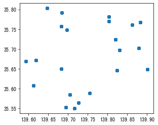
# ただの位置確認

figure()
subplot(111, aspect="equal")
plot(df["lon"], df["lat"], "o")
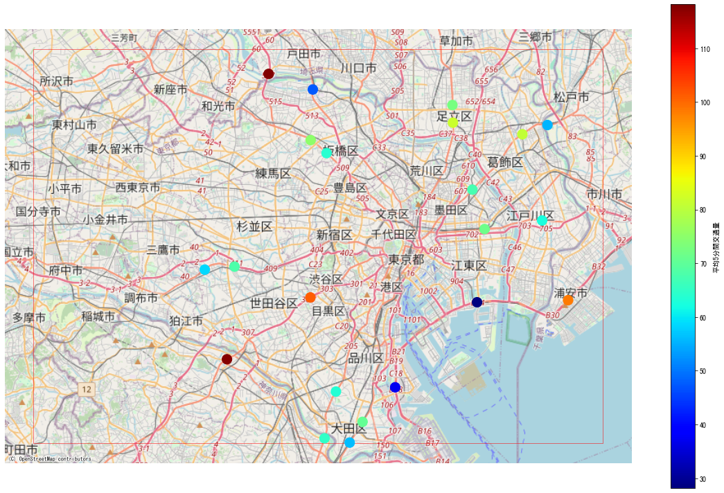
# OSMと合わせて平均交通量

import contextily as ctx
import geopandas as gpd
from shapely.geometry import box
from pyproj import Transformer

# 緯度経度のbboxを指定
min_lon, min_lat, max_lon, max_lat = min_x, min_y, max_x, max_y

# bboxからジオメトリを作成
bbox_geom = box(min_lon, min_lat, max_lon, max_lat)

# GeoDataFrameに変換(WGS84座標系)
gdf = gpd.GeoDataFrame(geometry=[bbox_geom], crs="EPSG:4326")

# Web Mercator座標系に変換(OSMタイルと合わせるため)
gdf = gdf.to_crs(epsg=3857)

# 交通データ
key = "traffic_up"
df_mean = df.groupby(["lon", "lat"], as_index=False)[key].mean()
transformer = Transformer.from_crs("EPSG:4326", "EPSG:3857", always_xy=True)
df_mean["x"], df_mean["y"] = transformer.transform(df_mean["lon"].values, df_mean["lat"].values)

# プロット
fig, ax = subplots(figsize=(16, 10))
gdf.plot(ax=ax, alpha=0.5, edgecolor='red', facecolor='none')

traffic_scat = ax.scatter(df_mean["x"], df_mean["y"], s=200, c=df_mean[key], cmap="jet")

# カラーバーを追加
cbar = fig.colorbar(traffic_scat, ax=ax)
cbar.set_label('平均5分間交通量')

# contextily でOSMタイルを追加
ctx.add_basemap(ax, source=ctx.providers.OpenStreetMap.Mapnik)

# 軸ラベルなどを設定
ax.set_axis_off()
tight_layout()
show()
# 時系列プロット

figure()
plot(df["datetime"], df["traffic_up"], "b.", alpha=0.1)
xlim([time_code_from_obj, time_code_to_obj])
ylabel("5分間交通量(上り)")
xlabel("日時")
figure()
plot(df["datetime"], df["traffic_down"], "r.", alpha=0.1)
xlim([time_code_from_obj, time_code_to_obj])
ylabel("5分間交通量(下り)")
xlabel("日時")
show()
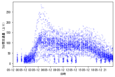
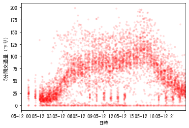
↑上りと下りで明らかにパターンが違うのがおもしろい
#下の3次元プロットをインタラクティブに動かす場合
#%matplotlib qt
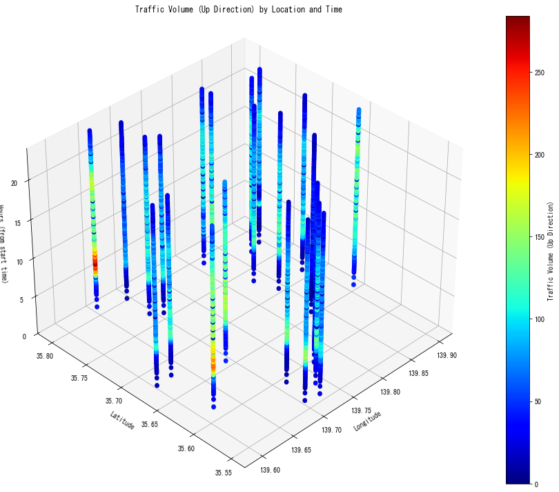
# 3次元時空間プロット

from mpl_toolkits.mplot3d import Axes3D

import matplotlib.pyplot as plt

# Create a 3D figure
fig = plt.figure(figsize=(14, 10))
ax = fig.add_subplot(111, projection='3d')

# Convert datetime to hours from midnight for better visualization
hours = [(dt - time_code_from_obj).total_seconds()/3600 for dt in df['datetime']]

# Create the scatter plot
scatter = ax.scatter(df['lon'], df['lat'], hours,
                    c=df['traffic_up'],
                    cmap='jet',
                    s=30)

# Add labels and title
ax.set_xlabel('Longitude')
ax.set_ylabel('Latitude')
ax.set_zlabel('Hours (from start time)')
ax.set_title('Traffic Volume (Up Direction) by Location and Time')

ax.set_zlim([0, (time_code_to_obj-time_code_from_obj).total_seconds()/3600])

# Add a color bar
cbar = plt.colorbar(scatter)
cbar.set_label('Traffic Volume (Up Direction)')

# Adjust the view angle for better visualization
ax.view_init(elev=35, azim=225)

plt.tight_layout()
plt.show()
データ出典・ライセンス
データの出典は以下です:交通量 API(国土交通省)機能による交通量(参考値)および国土交通省 API 機能による交通量(参考値)を加工して作成.交通量 API 機能を使用していますが、内容は国土交通省によって保証されたものではありません。
本コードのライセンスはパブリックドメイン(CC0)です.