はじめに
この記事は、Open Bandit Pipeline のアルゴリズム実装を行うことによりパッケージに採用されているアルゴリズムの理解を試みています。

先ずはこの記事の構成を示します。
- オープンソースの紹介 (Abstract: Open Bandit Dataset (OBD) & Open Bandit Pipeline (OBP))
- Open Bandit Pipeline のアルゴリズム実装 (実装)
2.1. Open Bandit Dataset (Open Bandit Dataset)
2.1.2. 必要なライブラリの読み込み
2.1.3. データの理解
2.2. Off-Policy Evaluation wih Open Bandit Pipeline([Open Bandit Pipeline] (#open-bandit-pipeline))
2.2.1. 意思決定 policy のオフラインシミュレーション
2.2.2. Contextual Logistic Thompson Sampling のオフライン評価
2.2.3. 信頼区間の算出
2.2.4. 性能の比較
- まとめ (まとめ)
- 参考資料 (参考資料)
Abstract: Open Bandit Dataset (OBD) & Open Bandit Pipeline (OBP)
株式会社ZOZOテクノロジーズに所属するZOZO研究所からバンディットに関する興味深いオープンソースが発表されています。
Open Bandit Dataset: https://research.zozo.com/data.html
Open Bandit Pipeline: https://github.com/st-tech/zr-obp/tree/master/obp
オープンソースの概要について論文とGitHubから抜粋します。
<Open Bandit Dataset>
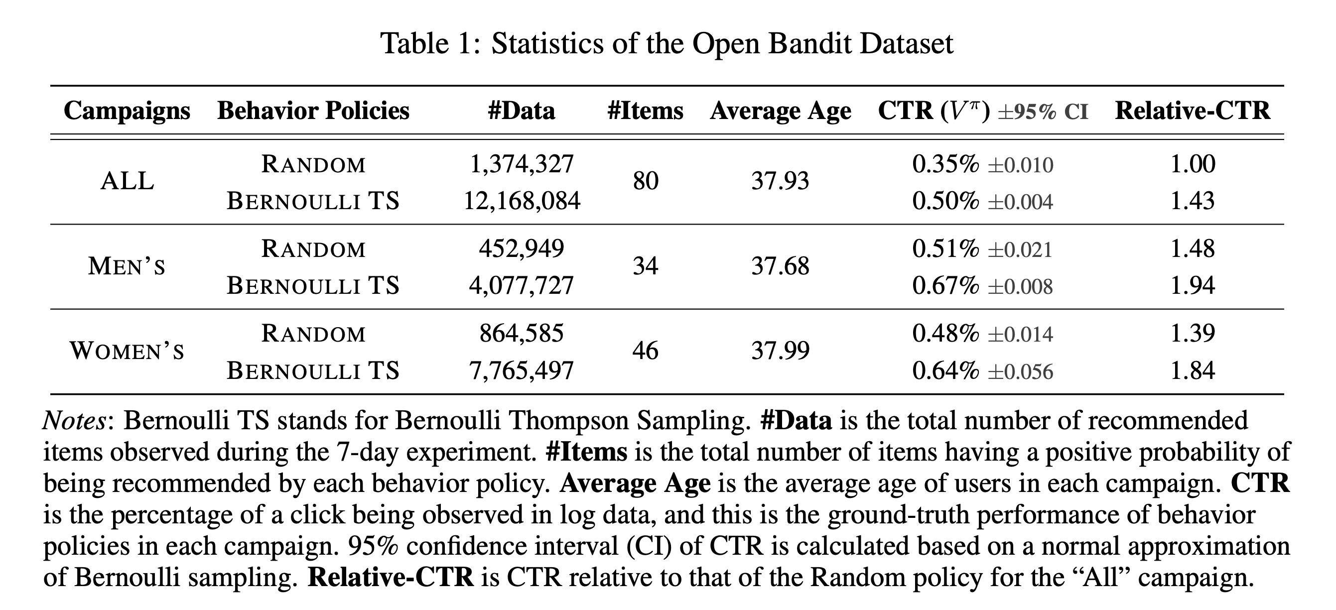
Our goal is to implement and evaluate OPE of bandit algorithms in realistic and reproducible ways. We release the Open Bandit Dataset, a logged bandit feedback collected on a large-scale fashion e-commerce platform, ZOZOTOWN.
When the platform produced the data, it used Bernoulli Thompson Sampling (Bernoulli TS) and Random policies to recommend fashion items to users. The dataset includes an A/B test of these policies and collected over 26 million records of users’ clicks and the ground-truth about the performance of BernoulliTS and Random.
To streamline and standardize the analysis of the Open Bandit Dataset, we also provide the Open Bandit Pipeline, a series of implementations of dataset preprocessing, behavior bandit policy simulators, and OPE estimators.
(A Large-scale Open Dataset for Bandit Algorithms)
<Open Bandit Pipeline>
Open Bandit Pipeline is a series of implementations of dataset preprocessing, offline bandit simulation, and evaluation of OPE estimators. This pipeline allows researchers to focus on building their OPE estimator and easily compare it with others’ methods in realistic and reproducible ways. Thus, it facilitates reproducible research on bandit algorithms and off-policy evaluation.
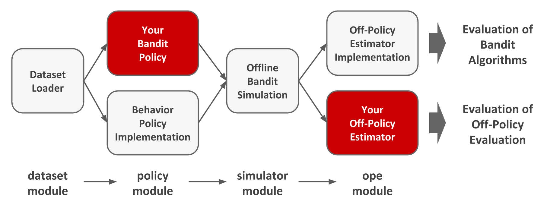
Structure of Open Bandit Pipeline
Open Bandit Pipeline consists of the following main modules.
◇dataset module: This module provides a data loader for Open Bandit Dataset and a flexible interface for handling logged bandit feedback. It also provides tools to generate synthetic bandit datasets.
◇policy module: This module provides interfaces for online and offline bandit algorithms. It also implements several standard algorithms.
◇simulator module: This module provides functions for conducting offline bandit simulation.
◇ope module: This module provides interfaces for OPE estimators. It also implements several standard OPE estimators.
(GitHub Open Bandit Pipeline)
モチベーションについてはZOZOテクノロジーズ TECH BLOG に丁寧な記載があるのでそちらを抜粋します。
機械学習は予測のための技術としてもてはやされています。実際多くの論文が、解く意味があるとされているタスクにおいてより良い予測精度を達成することを目指しています。もちろん予測値をそのまま活用する場面も多くあるでしょう。しかしとりわけウェブ産業における機械学習の応用場面に目を向けてみると、機械学習による予測値をそのまま使うのではなく、予測値に基づいて何かしらの意思決定を行っていることが多くあります。例えば、各ユーザーとアイテムのペアごとのクリック率を予測し、その予測値に基づいてユーザーごとにどのアイテムを推薦すべきか選択する。または、商品の購入確率予測に基づいてユーザーごとにどの商品の広告を提示するか決定する、などです。これらの例ではクリック率や購入確率の予測そのものよりもそれに基づいて作られる推薦や広告配信などの意思決定が重要です。
本記事の興味は、機械学習による予測値などに基づいて作られる意思決定policyの性能を評価することにあります。例えばクリック率の予測値に基づいてアイテム推薦の意思決定を行う場合、オフラインでクリック率の予測精度を評価指標としていることがあるでしょう。しかし、これは非直接的な評価方法です。予測値をそのままではなく何らかの意思決定を行うために用いているのならば、最終的に出来上がる意思決定policyの性能を直接評価するべきです。
意思決定policyの性能評価として理想的なのは、policyをサービスに実装してしまい興味があるKPIの挙動を見るというオンライン実験でしょう。しかし、何でもかんでもオンライン実験ができるわけではありません。なぜならば、オンライン実験には大きな実装コストが伴うからです。性能の悪い意思決定policyをオンライン実験してしまったときに、実験期間においてユーザー体験を害してしまったり、収入を減らしてしまう恐れもあります。従って、古い意思決定policyにより蓄積されたデータのみを用いて、新しい意思決定policyをオンラインに実装したときの性能を事前に見積もりたい、というモチベーションが生まれます。
このように、新たな意思決定policyの性能を過去の蓄積データを用いて推定する問題のことをOff-Policy Evaluation (OPE)と呼びます。NetflixやSpotify、Criteoなどの研究所がこぞってトップ国際会議でOPEに関する論文を発表しており、特にテック企業から大きな注目を集めています。正確なOPEは、多くの実務的メリットをもたらします。例えば、ある旧ロジックをそれとは異なる新ロジックに変えようと思ったとき、新ロジックがもたらすKPIの値を旧ロジックが蓄積したデータを用いて見積もることができます。また、ハイパーパラメータや機械学習アルゴリズムの組み合わせを変えることによって多数生成される意思決定policyの候補のうち、どれをオンライン実験に回すべきなのかを事前に絞り込むこともできます。
(Off-Policy Evaluationの基礎とZOZOTOWN大規模公開実データおよびパッケージ紹介)
実装
Open Bandit Pipeline のコードのアルゴリズム実装を行っていきます。
Open Bandit Dataset
扱うデータを取得します。
(今回は、大規模実験公開データと同質な少量データを GitHub から読み込み Cloud Storage のバケットにコピーしています。)
<Cloud Shell>
$ gcloud beta compute instances set-scopes git --scopes https://www.googleapis.com/auth/devstorage.read_write,trace --zone=<zone> --service-account=<service_account>
>> Updated [https://www.googleapis.com/compute/beta/projects/<project_id>/zones/<zone>/instances/git].

$ gcloud beta compute instances set-scopes git --scopes https://www.googleapis.com/auth/devstorage.full_control,trace --zone=<zone> --service-account=<service_account>
>> Updated [https://www.googleapis.com/compute/beta/projects/<project_id>/zones/<zone>/instances/git].
<Compute Engine VM>
$ ssh-keygen -t rsa

$ sudo apt-get install git
$ ssh -vT git@github.com
$ ssh -T git@github.com
$ git clone git@github.com:st-tech/zr-obp.git

$ gcloud auth login
$ gsutil cp -r /home/<user_name>/zr-obp/obd/bts/women gs://<bucket_name>
<必要なライブラリの読み込み>
import pandas as pd
import numpy as np
from tqdm import tqdm
from pathlib import Path
from dataclasses import dataclass
from obp.dataset import OpenBanditDataset
from obp.policy import LogisticTS
from obp.simulator import run_bandit_simulation
from obp.ope import (
    OffPolicyEvaluation,
    RegressionModel,
    ReplayMethod,
    DirectMethod,
    DoublyRobust,
    InverseProbabilityWeighting
)

from typing import Dict, Optional, Union
from sklearn.preprocessing import LabelEncoder
from sklearn.utils import check_random_state
from sklearn.ensemble import RandomForestClassifier as RandomForest
from scipy.optimize import minimize
<データの理解>
data_path = Path('.').resolve().parents[1] / 'python_code_/analysis_/Contextual'
# 「女性向けキャンペーン」において Bernoulli Thompson Sampling policyが集めたログデータを読み込む(これらは引数に設定)
# C:\Users\<user_name>\python_code_\analysis_\Contextual\bts\women\women.csv
dataset = OpenBanditDataset(behavior_policy = 'bts', campaign = 'women', data_path = data_path)
# 過去の意思決定policyによる蓄積データ`bandit feedback`を得る
bandit_feedback = dataset.obtain_batch_bandit_feedback()

print(bandit_feedback.keys())
>> dict_keys(['n_rounds', 'n_actions', 'action', 'position', 'reward', 'pscore', 'context', 'action_context'])
bandit_feedback は dataset(前回の Policy により得られたフィードバックデータ) から OPE に必要なデータを抽出し加工したデータです。
bandit_feedback は women.csv と item_context.csv から構成されています。
data = pd.read_csv('Contextual/bts/women/women.csv')
user_cols = data.columns.str.contains('user_feature')
context = pd.get_dummies(data.loc[:, user_cols], drop_first = True).values

item_context = pd.read_csv('Contextual/bts/women/item_context.csv')
item_feature_0 = item_context['item_feature_0']
item_feature_cat = item_context.drop(['item_feature_0', 'item_id'], axis = 1).apply(LabelEncoder().fit_transform)
action_context = pd.concat([item_feature_cat, item_feature_0], axis = 1).values

print(data.columns)
>> Index(['timestamp', 'item_id', 'position', 'click', 'propensity_score', 'user_feature_0', 'user_feature_1', 'user_feature_2',
'user_feature_3', 'user-item_affinity_0', 'user-item_affinity_1', 'user-item_affinity_2', 'user-item_affinity_3',
'user-item_affinity_4', 'user-item_affinity_5', 'user-item_affinity_6', 'user-item_affinity_7', 'user-item_affinity_8',
'user-item_affinity_9', 'user-item_affinity_10', 'user-item_affinity_11', 'user-item_affinity_12', 'user-item_affinity_13',
'user-item_affinity_14', 'user-item_affinity_15', 'user-item_affinity_16', 'user-item_affinity_17', 'user-item_affinity_18',
'user-item_affinity_19', 'user-item_affinity_20', 'user-item_affinity_21', 'user-item_affinity_22','user-item_affinity_23',
'user-item_affinity_24', 'user-item_affinity_25', 'user-item_affinity_26', 'user-item_affinity_27', 'user-item_affinity_28',
'user-item_affinity_29', 'user-item_affinity_30','user-item_affinity_31', 'user-item_affinity_32','user-item_affinity_33',
'user-item_affinity_34', 'user-item_affinity_35', 'user-item_affinity_36','user-item_affinity_37', 'user-item_affinity_38',
'user-item_affinity_39', 'user-item_affinity_40', 'user-item_affinity_41', 'user-item_affinity_42','user-item_affinity_43',
'user-item_affinity_44','user-item_affinity_45'], dtype='object')
print(item_context.columns)
>> Index(['item_id', 'item_feature_0', 'item_feature_1', 'item_feature_2', 'item_feature_3'], dtype='object')
bandit_feedback
◇n_rounds: サンプルサイズ
◇n_actions: クリエイティブ数(クリエイティブの候補)
◇action: バンディットアルゴリズムにより選択されたクリエイティブ
◇position: クリエイティブの表示位置(今回は3ヵ所の候補があるとしています)
◇reward: 報酬(not CV: 0 / CV: 1)
◇pscore: Propensity Score
◇context: ダミー変数化されたユーザー特徴量
◇action_context: item_context から item_id を除いたデータ
women.csv
◇timestamp: timestamps of impressions.
◇item_id: index of items as arms (index ranges from 0-80 in "All" campaign, 0-33 for "Men" campaign, and 0-46 "Women" campaign).
◇position: the position of an item being recommended (1, 2, or 3 correspond to left, center, and right position of the ZOZOTOWN recommendation interface, respectively).
◇click: target variable that indicates if an item was clicked (1) or not (0).
◇propensity_score: the probability of an item being recommended at each position.
◇user feature 0-4: user-related feature values.
◇user-item affinity 0-: user-item affinity scores induced by the number of past clicks observed between each user-item pair.
item_context.csv
◇item_id: index of items as arms (index ranges from 0-80 in "All" campaign, 0-33 for "Men" campaign, and 0-46 "Women" campaign).
◇item feature 0-3: item related feature values
Open Bandit Pipeline
「旧ロジックである Bernoulli Thompson Sampling policy が収集した過去データを用いて、新ロジックである Contextual Logstic Thompson Sampling policy の性能をオフライン評価する」という例を用います。
このセクションでは Open Bandit Pipeline とアルゴリズム実装それぞれのコードを順に載せていきます。
<意思決定 policy のオフラインシミュレーション>
前回の意思決定 policy により得られたフィードバックデータを新しい意思決定 policy におけるアルゴリズム(Contextual Logistic Thompson Sampling)に学習させることでシミュレーションを行います。
<Open Bandit Pipeline>
counterfactual_policy = LogisticTS(n_actions = dataset.n_actions, len_list = dataset.len_list,
                                    random_state = 0, dim = bandit_feedback['context'].shape[1])
selected_actions = run_bandit_simulation(bandit_feedback = bandit_feedback, policy = counterfactual_policy)
>> 100%|███████████████████████████████████████████████████████████████████████████| 10000/10000 [00:13<00:00, 739.71it/s]

print(selected_actions )
>> array([[45, 11, 20],
          [45, 11, 20],
          [45, 11, 20],
          ...,
          [26, 22, 10],
          [29, 15,  6],
          [26, 22, 10]], dtype=int64)
dim = 19 # bandit_feedback["context"].shape[1]
n_actions = 46
len_list = 3
batch_size = 1
alpha = 1.0
beta = 1.0
lambda_ = 1.0
random_state = 0

reward_counts = np.zeros(n_actions)
action_counts = np.zeros(n_actions, dtype=int)

for key_ in ['action', 'position', 'reward', 'pscore', 'context']:
    if key_ not in bandit_feedback:
        raise RuntimeError(f"Missing key of {key_} in 'bandit_feedback'.")

context = bandit_feedback['context']
action = bandit_feedback['action']
reward = bandit_feedback["reward"]
position = bandit_feedback["position"]
pscore = bandit_feedback["pscore"]

n_trial = 0
action_counts_temp = np.zeros(n_actions, dtype = int)
reward_counts_temp = np.zeros(n_actions)

selected_actions_list = list()
dim_context = bandit_feedback["context"].shape[1]

reward_lists = [[] for _ in np.arange(n_actions)]
context_lists = [[] for _ in np.arange(n_actions)]

# policy_type = "contextfree"
policy_type = "contextual"

@dataclass
class Model:
    """MiniBatch Online Logistic Regression Model."""
    lambda_: float
    alpha: float
    dim: int
    random_state: Optional[int] = None

    def __post_init__(self) -> None:
        """Initialize Class."""
        self._m = np.zeros(self.dim)
        self._q = np.ones(self.dim) * self.lambda_
        self.random_ = check_random_state(self.random_state)

    def predict_proba_with_sampling(self, X: np.ndarray) -> np.ndarray:
        """Predict extected probability by the sampled coefficient."""
        return sigmoid(X.dot(self.sample_()))

    def sample_(self) -> np.ndarray:
        """Sample coefficient vector from the prior distribution."""
        sd = self.alpha * self._q ** (-1.0)
        return self.random_.normal(self._m, sd, size = self.dim)

    def fit(self, X: np.ndarray, y: np.ndarray):
        """Update coefficient vector by the mini-batch data."""
        self._m = minimize(
            fun = loss,
            x0 = self._m,
            args = (X, y, self._q, self._m),
            jac = grad,
            method="L-BFGS-B",
            options={"maxiter": 20, "disp": False}
        ).x

        P = (1 + np.exp(1 + X.dot(self._m))) ** (-1)
        self._q = self._q + (P * (1 - P)).dot(X ** 2)

def sigmoid(x: Union[float, np.ndarray]) -> Union[float, np.ndarray]:
        """Calculate sigmoid function."""
        return 1.0 / (1.0 + np.exp(-x))

def loss(w: np.ndarray, *args) -> float:
    """Calculate loss function."""
    X, y, _q, _m = args
    return 0.5 * (_q * (w - _m)).dot(w - _m) + np.log(1 + np.exp(-y * w.dot(X.T))).sum()

def grad(w: np.ndarray, *args) -> np.ndarray:
    """Calculate gradient."""
    X, y, _q, _m = args
    return _q * (w - _m) + (-1) * (((y * X.T) / (1.0 + np.exp(y * w.dot(X.T)))).T).sum(axis=0)

alpha_list = alpha * np.ones(n_actions)
lambda_list = lambda_ * np.ones(n_actions)

model_list = [
    Model(
        lambda_ = lambda_list[i],
        alpha = alpha_list[i],
        dim = 19,
        random_state = 0,
    )
    for i in np.arange(n_actions)
]

for action_, reward_, position_, context_ in tqdm(
    zip(bandit_feedback["action"],
        bandit_feedback["reward"],
        bandit_feedback["position"],
        bandit_feedback["context"],
       ),
    total = bandit_feedback['n_rounds'],
):
    if policy_type == "contextfree":
        # Returns
        # selected_actions: array-like shape (len_list, )
        # List of selected actions.
        predicted_rewards = random_.beta(
            a = reward_counts + alpha,
            b = (action_counts - reward_counts) + beta,
        )
        selected_actions = predicted_rewards.argsort()[::-1][: len_list]

    elif policy_type == "contextual":
        # Returns
        # selected_actions: array-like shape (len_list, )
        # List of selected actions.
        theta = np.array(
            [model.predict_proba_with_sampling(context_.reshape(1, dim_context)) for model in model_list]
        ).flatten()
        selected_actions = theta.argsort()[::-1][: len_list]

    action_match_ = action_ == selected_actions[position_]

    if action_match_:
        if policy_type == "contextfree":
            n_trial += 1
            action_counts_temp[action_] += 1
            reward_counts_temp[action_] += reward_
            # batch update
            if n_trial % batch_size == 0:
                action_counts = np.copy(action_counts_temp)
                reward_counts = np.copy(reward_counts_temp)

        elif policy_type == "contextual":
            n_trial += 1
            action_counts[action_] += 1
            reward_lists[action_].append(reward_)
            context_lists[action_].append(context_.reshape(1, dim_context))
            if n_trial % batch_size == 0:
                for action, model in enumerate(model_list):
                    if not len(reward_lists[action]) == 0:
                        model.fit(
                            X = np.concatenate(context_lists[action], axis=0),
                            y = np.array(reward_lists[action]),
                        )
                reward_lists = [[] for _ in np.arange(n_actions)]
                context_lists = [[] for _ in np.arange(n_actions)]

    selected_actions_list.append(selected_actions)
>> 100%|███████████████████████████████████████████████████████████████████████████| 10000/10000 [00:13<00:00, 739.71it/s]

selected_actions_list = np.array(selected_actions_list)
print(selected_actions_list)
>> array([[45, 11, 20],
          [45, 11, 20],
          [45, 11, 20],
          ...,
          [26, 22, 10],
          [29, 15,  6],
          [26, 22, 10]], dtype=int64)
文脈付きバンディット問題を扱っているため policy_type = "contextual" が設定されており if 文の条件分岐では policy_type == "contextual" が選択されます。
今回の実装に用いている例では、Contextual Thompson Sampling はユーザーごとに報酬構造が変化することを仮定した上で各クリエイティブの選択において期待値の最大化を図るアルゴリズムです。
今回はロジスティック回帰においてシグモイド関数を用いているため解析的にパラメータを求めることは難しくラプラス近似を行います。
上記のコードから、シグモイド関数のパラメータ更新のために対数尤度を2次近似した目的関数の最小化問題を解いていると解釈できます。
loss 関数の数式は2次近似を行った目的関数(ニュートン法により求まった MAP 推定量の周りで負の対数尤度を2次近似した関数)であり (np.log(1 + np.exp(-y * w.dot(X.T)))).sum() の部分はロジスティック回帰における負の対数尤度を表しています。 grad 関数の数式は minimize 関数(L-BFGS-B を指定することでニュートン法により多変数関数における最適化を実行)における最適化の際に勾配方向にパラメータを更新するために必要なヤコビアンを表しています。
loss 関数に対しての最適化問題を解くことでシグモイド関数のパラメータの事後分布に近似させる正規分布に必要なパラメータ(_m: ニュートン法により求められる MAP 推定量, sd: ヘッセ行列 _q の逆行列を持つ標準偏差)を算出しています。
sample 関数の正規分布からサンプリングされた値を更新されたパラメータとして sigmoid 関数が受け取ります。
Open Bandit Pipeline では LogisticTS クラスを宣言するとクリエイティブの数だけロジスティック回帰モデルが生成されます。アルゴリズム実装コードの model_list にあたります。
モデルの更新は if n_trial % batch_size == 0 をトリガーとして fit 関数により行われています。
batch_size = 1 を設定しているため for 文により各ユーザーのフィードバックデータが流れてくる度にモデルを更新していく仕組みです。
各クリエイティブに対応するモデル、今回であれば 0 から 45 までの 46 のモデルに対し報酬を受け取ったクリエイティブに対応するモデルを更新します。アルゴリズム実装コードの if not len(reward_lists[action]) == 0 にあたります。
更新の際にはラプラス近似を行うため、各ユーザーのフィードバックデータにおいて報酬を受け取ったクリエイティブ(選択されたクリエイティブ)番号に対応する context_lists:X (ユーザー特徴量) と reward_lists: y (予測対象である報酬) を引数として与えシグモイド関数のパラメータの更新が行われています。
predict_proba_with_sampling 関数によりユーザーの特徴量に対し各モデルにおいて reward = 1 となる確率を予測し確率の高いクリエイティブの上位 3 つを selected_actions_list に格納します。
<Contextual Logistic Thompson Sampling のオフライン評価>
シュミレーションの結果に基づき、Doubly Robust を用いて Contextual Logistic Thompson Sampling のオフライン評価(OPE)を行います。
<Open Bandit Pipeline>
ope = OffPolicyEvaluation(
    bandit_feedback = bandit_feedback,
    regression_model = RegressionModel(base_model = RandomForest(n_estimators = 100, random_state = 0)),
    action_context = dataset.action_context,
    ope_estimators = [DoublyRobust()]
)
estimator_inputs = ope._create_estimator_inputs(selected_actions = selected_actions)
print(estimator_inputs)
>> {'reward': array([0, 0, 0, ..., 0, 0, 0], dtype=int64),
    'pscore': array([0.02173913, 0.023865  , 0.02101   , ..., 0.0102    , 0.00839, 0.016595  ]),
    'action_match': array([False, False, False, ..., False, False, False]),
    'estimated_rewards_by_reg_model': array([0., 0., 0., ..., 0., 0., 0.])}

estimated_policy_value = ope.estimate_policy_values(selected_actions = selected_actions)
print(estimated_policy_value)
>> {'dr': 0.0009044371394456017}
def create_estimator_inputs(selected_actions_list: np.ndarray) -> Dict[str, np.ndarray]:
    """Create input dictionary to estimate policy value"""
    estimator_inputs = {
        input_: bandit_feedback[input_] for input_ in ['reward', 'pscore']
                       }
    estimator_inputs['action_match'] = (
        bandit_feedback['action'] == selected_actions_list[np.arange(bandit_feedback['n_rounds']),
                                                      bandit_feedback['position']
                                                     ]
    )
    regression_model = True
    if regression_model == True:
        context = bandit_feedback["context"]
        position = bandit_feedback["position"]
        action = bandit_feedback['action']

        selected_actions_at_positions = selected_actions_list[np.arange(position.shape[0]), position]

        base_model = RandomForest(n_estimators = 100, random_state = 0)
        X = np.c_[context, action_context[action]]
        X_ = np.c_[context, action_context[selected_actions_at_positions]]
        fitting_method = 'normal'
        if fitting_method == "normal":
            # Method to fit the regression method.
            base_model.fit(X, bandit_feedback['reward'])
            estimator_inputs[
                "estimated_rewards_by_reg_model"
            ] = base_model.predict_proba(X_)[:, 1]

        elif fitting_method == 'iw':
            # Method to fit the regression method.
            # 'iw' stands for importance weighting.
            sample_weight = np.mean(bandit_feedback['pscore']) / bandit_feedback['pscore']
            base_model.fit(X, bandit_feedback['reward'], sample_weight = sample_weight)
            estimator_inputs[
                "estimated_rewards_by_reg_model"
            ] = base_model.predict_proba(X_)[:, 1]

        elif fitting_method == 'mrdr':
            # Method to fit the regression method.
            # 'mrdr' stands for more robust doubly robust.
            sample_weight = (1.0 - bandit_feedback['pscore']) / bandit_feedback['pscore'] ** 2
            base_model.fit(X, bandit_feedback['reward'], sample_weight = sample_weight)
            estimator_inputs[
                "estimated_rewards_by_reg_model"
            ] = base_model.predict_proba(X_)[:, 1]

        return estimator_inputs

def estimate_policy_values(selected_actions_list: np.ndarray, method) -> Dict[str, float]:
    """Estimate policy value of a counterfactual policy."""
    policy_value_dict = dict()
    estimator_inputs = create_estimator_inputs(
        selected_actions_list = selected_actions_list
    )
    if method == 'DirectMethod':
        # DirectMethod
        policy_value_dict['DirectMethod'] = np.mean(estimator_inputs['estimated_rewards_by_reg_model'])

    if method == 'InverseProbabilityWeighting' :
        # InverseProbabilityWeighting
        estimated_rewards = (estimator_inputs['action_match'] * estimator_inputs['reward']) / estimator_inputs['pscore']
        policy_value_dict['InverseProbabilityWeighting'] = np.mean(estimated_rewards)

    elif method == 'DoublyRobust':
        # DoublyRobust
        estimated_rewards = (
            (estimator_inputs['action_match'] * (estimator_inputs['reward'] - estimator_inputs['estimated_rewards_by_reg_model'])) / estimator_inputs['pscore']
        ) + estimator_inputs['estimated_rewards_by_reg_model']
        policy_value_dict['DoublyRobust'] = np.mean(estimated_rewards)

    return estimated_rewards, policy_value_dict


estimator_inputs = create_estimator_inputs(selected_actions_list = selected_actions_list)
print(estimator_inputs)
>> {'reward': array([0, 0, 0, ..., 0, 0, 0], dtype=int64),
    'pscore': array([0.02173913, 0.023865  , 0.02101   , ..., 0.0102    , 0.00839, 0.016595  ]),
    'action_match': array([False, False, False, ..., False, False, False]),
    'estimated_rewards_by_reg_model': array([0., 0., 0., ..., 0., 0., 0.])}

estimated_policy_value = estimate_policy_values(selected_actions_list, method = 'DoublyRobust')
print(estimated_policy_value[0])
>> array([0., 0., 0., ..., 0., 0., 0.])
print(estimated_policy_value[1])
>> {'DoublyRobust': 0.0009044371394456017}
<OffPolicyEvaluation>
Open Bandit Pipeline では OffPolicyEvaluation クラスを宣言すると base_model として設定した RandomForest に対し fit と predict_proba を実行します。 OffPolicyEvaluation クラスを宣言する際の引数 RegressionModel に fitting_method を引数として渡していないためデフォルト値の fitting_method = "normal" が選択されています。アルゴリズム実装コードの if fitting_method == "normal" にあたります。
fit はフィードバックデータの「ユーザー特徴量(context)と各ユーザーに対して選択されたクリエイティブの特徴量(action_context[action])」を入力として「報酬(bandit_feedback['reward'])」を予測したモデルを返します。
<\_create_estimator_inputs>
Open Bandit Pipeline の _create_estimator_inputs 関数は estimate_policy_values に必要なデータが格納された estimator_inputs を返します。 OffPolicyEvaluation クラスと _create_estimator_inputs 関数 はどちらもアルゴリズム実装コードの create_estimator_inputs にあたります。
predict_proba は「フィードバックデータのユーザー特徴量(context)と各ユーザーに対して Contextual Logistic Thompson Sampling により選択されたクリエイティブの特徴量(selected_actions_at_positions)」を入力として「期待される報酬(not CV: 0 / CV: 1)それぞれの確率」を返します。
predict_proba により得られた reward = 1 (CV = 1) となる確率を estimated_rewards_by_reg_model として estimator_inputs に格納しています。
action_match は前回の意思決定 policy により選択されたクリエイティブと Contextual Logistic Thompson Sampling により選択されたクリエイティブが同じであるか否かに対応する True または False からなるデータです。
<estimate_policy_values>
Open Bandit Pipeline の estimate_policy_values では Contextual Logistic Thompson Sampling のオフライン評価(OPE)を行います。
つまり、前回の意思決定 policy に対して新しい意思決定 policy はどの程度の性能を有するのかについて評価を行います。
論文では ground-truth に対して「Direct Method(DM)」「Inverse Probability Weighting(IPW)」「Doubly Robust(DR)」による評価の比較が行われていますが今回は Doubly Robust のみを実装しています。アルゴリズム実装コードには DM と IPW のアルゴリズムも載せてあるので引数 method に ['Direct Method', 'InverseProbabilityWeighting', 'DoublyRobust'] を渡せば評価を比較することができます。
DM は報酬の真の期待値と推定値とが大きく異なる場合にバイアスが大きくなり、IPW は前回の意思決定 policy と新しい意思決定 policy の性能が大きく異なる場合やサンプルサイズが小さい場合にバリアンスが大きくなる傾向にあります。ただしサンプルサイズが大きい場合には IPW は普遍推定量であるため A/Bテスト に近似されます。
DM と IPW の折衷案にあたるのが DR です。
DR は「IPW(${\pi_k}$ の推定精度に大きく依存するという意味で介入を予測する回帰モデル)」と「DR(${\hat{\mu}}$ の推定精度に大きく依存するという意味で結果変数(報酬)を予測する回帰モデル)」のどちらかが正確であれば結果変数(報酬)の真の期待値に対し一致推定量として扱えます。
ただしその条件を満たしていなければ IPW よりも性能が劣る(MSE の値が高い)ことがあります。
estimate_policy_values の DoublyRobust に関してより具体的には以下の数式を計算しています。
\begin{aligned}\widehat{V}_{DR}^\pi(\pi;D) = \frac{1}{T} \sum_{t = 1}^{T}\sum_{a = 1}^{m} \Big\{ ({Y_t - \hat{\mu}(a_t|X_t))D_{ta} \frac{\pi(a_t|X_t)}{\pi{_b(a_t|X_t)}} } + \pi(a_t|X_t)\hat{\mu}(a_t|X_t) \Big\} \end{aligned}
\\
where \ D = { \{ {x_t}, {a_t}, {Y_t} \} }_{t = 1}^T
• ${\hat{\mu}}$ is independent of ${z_n}$.
• ${\pi_k}$ is conditionally independent of $\{x_l, a_l, Y_l \}_{l\geq{k}}$ conditioned on ${z_{k-1}}$.
(${z_k = (x_1, a_1, Y_1,...,x_k, a_k, Y_k)}$)
The first assumption means that ${\hat{\mu}}$ can be assumed fixed and determined before we see the input data ${z_n}$, for example, by initially splitting the input dataset and using the first part to obtain ${\hat{\mu}}$ and the second part to evaluate the policy. In our analysis, we condition on ${\hat{\mu}}$ and ignore any randomness in its choice.
The second assumption means that ${\pi_k}$ is not allowed to depend on future. A simple way to satisfy this assumption is to split the dataset to form an estimator (and potentially also include data ${z_{k-1}}$).
If we have some control over the exploration process, we might also have access to “perfect logging”, that is, recorded probabilities ${\pi_{k}(a_k|x_k)}$. With perfect logging, we can achieve ${\hat\pi_k = \pi_{k}}$, respecting our assumptions.
${D}$ は過去の意思決定 policy から得られるデータです。
つまり、観測される特徴量ごとに過去の意思決定 policy における行動は ${a_t ∼ \pi_b(⋅|x_{t})}$ により選択されており結果として潜在目的変数 ${Y_t = Y_t(a_t)}$ が観測されることでサンプルサイズ ${T}$ のフィードバックデータが構成されることを意味しています。
完璧な推定を行うことは実際には難しく、「介入を予測する回帰モデルと結果変数(報酬)を予測する回帰モデルとして振る舞う」${\widehat{V}_{DR}^\pi}$ が真の値からどれだけ離れているかに興味があります。
より詳しいことは ZOZOテクノロジーズ TECH BLOG の記事(Off-Policy Evaluationの基礎とZOZOTOWN大規模公開実データおよびパッケージ紹介)や論文(Doubly Robust Policy Evaluation and Optimization)に記載されています。
<信頼区間の算出>
ブートストラップ法(推定量に対しリサンプリングを行うことで母集団からの標本抽出を疑似的に再現)により信頼区間(真の値が取り得る範囲)を算出します。
<Open Bandit Pipeline>
estimated_policy_value, estimated_interval = ope.summarize_off_policy_estimates(selected_actions = selected_actions_list, random_state = 0)

print(estimated_policy_value)
>>
    estimated_policy_value
dr  0.000904

print(estimated_interval )
>>
    95.0% CI (lower) 95.0% CI (upper)     mean
dr  -0.00105         0.00215	      0.000765
def estimate_confidence_interval_by_bootstrap(alpha, n_boostrap_samples, random_state ):
    boot_samples = list()
    random_ = check_random_state(random_state)

    estimator_inputs = create_estimator_inputs(selected_actions_list = selected_actions_list)
    estimated_policy_value = estimate_policy_values(selected_actions_list, method = 'DoublyRobust')

    samples = estimated_policy_value[0]

    for _ in np.arange(n_boostrap_samples):
        boot_samples.append(np.mean(random_.choice(samples, size = samples.shape[0])))

    lower_bound = np.percentile(boot_samples, 100 * (alpha / 2))
    upper_bound = np.percentile(boot_samples, 100 * (1.0 - alpha / 2))

    return {
        'mean': np.mean(boot_samples),
        f"{100 * (1. - alpha)}% CI (lower)": lower_bound,
        f"{100 * (1. - alpha)}% CI (upper)": upper_bound
    }


print(estimate_confidence_interval_by_bootstrap(alpha = 0.05, n_boostrap_samples = 100, random_state = 0))
>> {'mean': 0.0007653177020632711,
    '95.0% CI (lower)': -0.0010498451155268806,
    '95.0% CI (upper)': 0.002150102018984923}
ブートストラップ法はリサンプリング回数が 100 のような少ない回数であったとしてもサンプルサイズが大きい場合には精度が高くなります。
今回は n_boostrap_samples = 100 を設定しており DR により得られた Contextual Logistic Thompson Sampling の性能の推定値に対し 95% 信頼区間を算出しています。
Open Bandit Pipeline では visualize_off_policy_estimates 関数を用いることで信頼区間の幅を seaborn の barplot で表示することができます。今回であれば barplot の引数である ci と n_boot にはそれぞれ 0.95 と 100 が渡されます。
<性能の比較>
意思決定 policy における旧ロジック(Bernoulli Thompson Sampling)と新ロジック(Contextual Logistic Thompson Sampling)の性能を比較します。
relative_policy_value_of_contextual_logistic_ts = estimated_policy_value[1]['DoublyRobust'] / bandit_feedback['reward'].mean()

pritn(relative_policy_value_of_contextual_logistic_ts )
>> 0.19661676944469603
新ロジックの性能は OPE(DR) による推定値を、旧ロジックの性能はフィードバックデータの報酬の平均をとることで推定できる真の値を用いています。
結果として、新ロジック(Contextual Logistic Thompson Sampling)の性能は旧ロジック(Bernoulli Thompson Sampling)と比較して 19.66% 上回ると推定されています。
まとめ
Open Bandit Pipeline のアルゴリズムを実装してみました。
コードや数学に関しての間違いなどありましたらご指摘のほどよろしくお願いいたします。
参考資料
<論文>
A Large-scale Open Dataset for Bandit Algorithms (Yuta Saito, Shunsuke Aihara, Megumi Matsutani, Yusuke Narita)
An Empirical Evaluation of Thompson Sampling (Olivier Chapelle, Lihong Li)
Doubly Robust Policy Evaluation and Optimization (Miroslav Dud´ık, Dumitru Erhan, John Langford and Lihong Li)
<サイト>
Contextual Bandits in Recommendation (James Mclnerney)
Off-Policy Evaluationの基礎とZOZOTOWN大規模公開実データおよびパッケージ紹介 (齋藤 優太)
ZOZO研究所、ZOZOTOWNのファッション推薦データとアルゴリズム研究開発基盤をオープンソースで公開
バンディットアルゴリズムと因果推論 / Bandit Algorithm And Casual Inference (安井 翔太)
最急降下法による非線形最適化MATLAB&Pythonサンプルプログラム
ロボティクスにおける線形代数
<GitHub>
Open Bandit Dataset
Open Bandit Pipeline
description of「Open Bandit Dataset and Open Bandit Pipeline」