サポートベクトルマシン(SVM)とは?
-
「マージン最大化」と呼ばれる考えに基づき、主に2値の分類問題に使われる。(多クラス分類、回帰問題への拡張も可能)
-
計算コストが比較的大きいため、大規模なデータセットには適していない。よって、主に中小規模のデータセットで使われる。
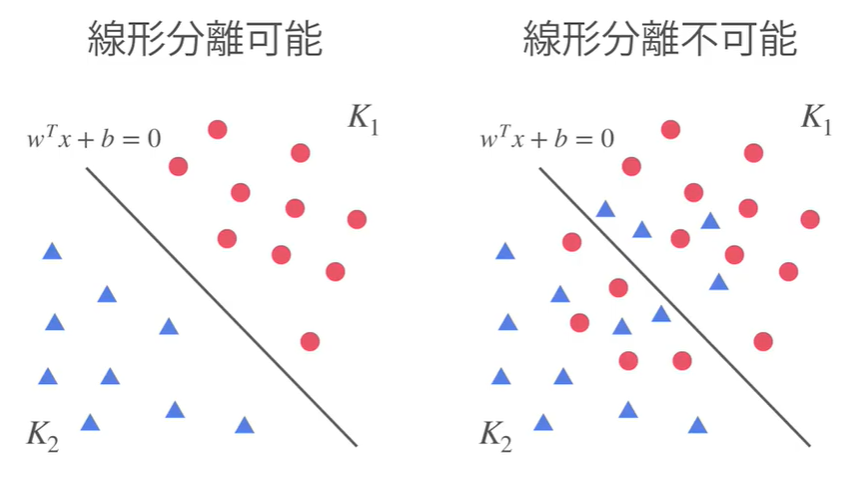
線形分離可能とは?
直線でクラス分類が可能か否か。
-
線形分離可能な場合、ハードマージンSVM
-
線形分離不可能な場合、ソフトマージンSVM
と呼ぶ。
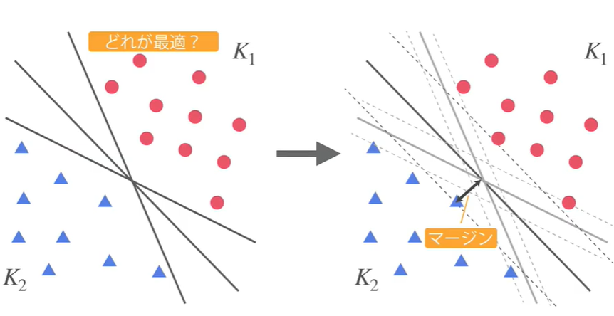
「マージン最大化」のイメージ(線形分離可能)
分割した直線から最も近い点までの距離をマージンと呼ぶ。
その最も近い点をサポートベクトルと呼ぶ。
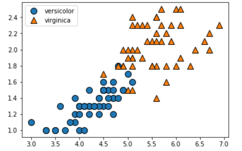
実験①
import mglearn
import numpy as np
import pandas as pd
import matplotlib.pyplot as plt
from sklearn.datasets import load_iris

iris=load_iris()
X=iris.data[50:,2:] #target=0or1or2
y=iris.target[50:]-1


mglearn.discrete_scatter(X[:,0],X[:,1],y)#第1引数…xの1番目の特徴量,第2引数…xの2番目の特徴量,第3引数…正解ラベル
plt.legend(["versicolor","virginica"],loc="best")
plt.show()
ハイパーパラメータを操作(C=1 or C=100)
from sklearn.svm import LinearSVC
from sklearn.model_selection import train_test_split

X_train,X_test,y_train,y_test=train_test_split(X,y,random_state=0)

svm=LinearSVC(C=1.0).fit(X_train,y_train)

def plot_separator(model):
    plt.figure(figsize=(10,6))
    mglearn.plots.plot_2d_separator(model,X)
    mglearn.discrete_scatter(X[:,0],X[:,1],y)
    plt.xlabel("petal length")
    plt.ylabel("petal width")
    plt.show()

plot_separator(svm)

# Cが大きい→ハードマージンSVMに近づく
# Cが小さい→誤分類を許容しやすい
svm_100=LinearSVC(C=100).fit(X_train,y_train) #default=1
plot_separator(svm_100)


print("score on training set :{:.2f}".format(svm.score(X_train,y_train)))
print("score on test set :{:.2f}".format(svm.score(X_test,y_test)))

print("score on training set :{:.2f}".format(svm_100.score(X_train,y_train)))
print("score on test set :{:.2f}".format(svm_100.score(X_test,y_test)))

実験②
import mglearn
import numpy as np
import pandas as pd
import matplotlib.pyplot as plt
from sklearn.datasets import make_moons

moons=make_moons(n_samples=200,noise=0.1,random_state=0)

X=moons[0]
y=moons[1]

plt.figure(figsize=(12,8))
mglearn.discrete_scatter(X[:,0],X[:,1],y)
plt.plot()
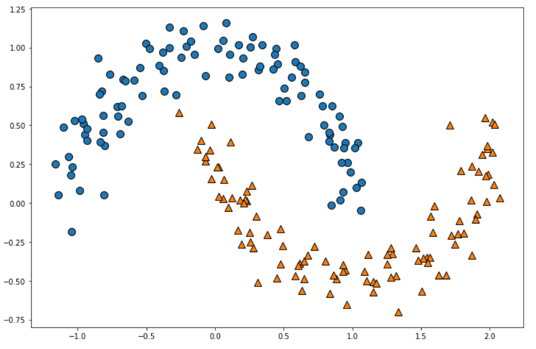
実験①とは異なる二値分布になりました。
from sklearn.svm import LinearSVC
from sklearn.model_selection import train_test_split
from sklearn.preprocessing import StandardScaler

scaler=StandardScaler()
X_scaled=scaler.fit_transform(X)

X_train,X_test,y_train,y_test=train_test_split(X,y,random_state=0)

lin_svm=LinearSVC().fit(X_train,y_train)

plt.figure(figsize=(12,8))
mglearn.plots.plot_2d_separator(lin_svm,X)
mglearn.discrete_scatter(X[:,0],X[:,1],y)
plt.xlabel("$x_0$",fontsize=20)
plt.ylabel("$x_1$",fontsize=20)
plt.show()
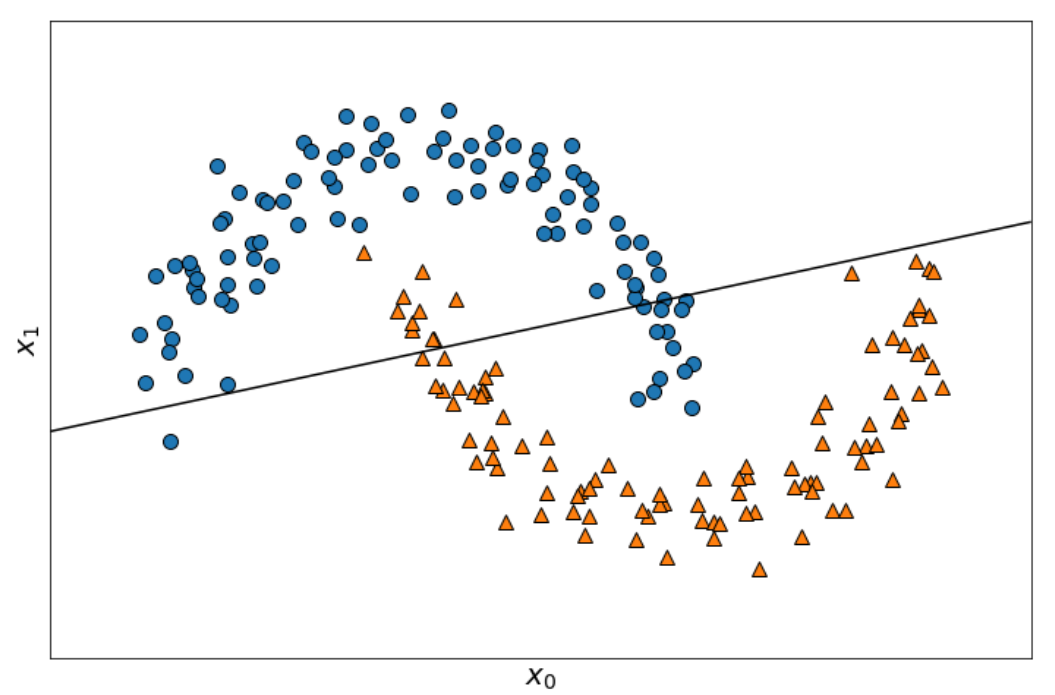
線形分離できていないことがはっきり分かりますね。
高次元特徴量空間生成
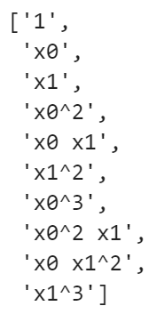
from sklearn.preprocessing import PolynomialFeatures

poly = PolynomialFeatures(degree=3)
X_train_poly=poly.fit_transform(X_train)
X_test_poly=poly.fit_transform(X_test)

# 10次元まで拡張できたことを確認
poly.get_feature_names()
標準化
X_train_poly_scaled=scaler.fit_transform(X_train_poly)
X_test_poly_scaled=scaler.fit_transform(X_test_poly)

lin_svm = LinearSVC().fit(X_train_poly_scaled,y_train)
# コードが楽になるバージョン
from sklearn.pipeline import Pipeline

poly_svm=Pipeline([
    ("poly",PolynomialFeatures(degree=3)),
    ("scaler",StandardScaler()),
    ("svm",LinearSVC())
])
poly_svm.fit(X,y)
def plot_decision_function(model):
    _x0 = np.linspace(-1.5,2.5,100)
    _x1 = np.linspace(-1.0,1.5,100)
    x0,x1 = np.meshgrid(_x0,_x1)
    X=np.c_[x0.ravel(),x1.ravel()]
    y_pred=model.predict(X).reshape(x0.shape)
    y_decision=model.decision_function(X).reshape(x0.shape)
    plt.contourf(x0,x1,y_pred,cmap=plt.cm.brg,alpha=0.2)
    plt.contourf(x0,x1,y_decision,lavels=[y_decision.min(),0,y_decision.max()],alpha=0.3)

def plot_dataset(X,y):
    plt.plot(X[:,0][y==0],X[:,1][y==0],"bo",ms=15)
    plt.plot(X[:,0][y==1],X[:,1][y==1],"r^",ms=15)
    plt.xlabel("$x_1$",fontsize=20)
    plt.ylabel("$x_2$",fontsize=20,rotation=0)

plt.figure(figsize=(12,8))
plot_decision_function(poly_svm)
plot_dataset(X,y)
plt.show()

カーネル法を用いて計算負荷量軽減
カーネル法は高次元特徴量を計算する際に計算量を軽減してくれるもの。(内積計算が得意)
from sklearn.svm import SVC

kernel_svm=Pipeline([
    ("scaler",StandardScaler()),
    ("svm",SVC(kernel="poly",degree=3,coef0=1))#poly=多項式
])

kernel_svm.fit(X,y)

plt.figure(figsize=(12,8))
plot_decision_function(kernel_svm)
plot_dataset(X,y)
plt.show()

可視化
def plot_decision_function(model):
    _x0 = np.linspace(-1.5,2.5,100)
    _x1 = np.linspace(-1.0,1.5,100)
    x0,x1 = np.meshgrid(_x0,_x1)
    X=np.c_[x0.ravel(),x1.ravel()]
    y_pred=model.predict(X).reshape(x0.shape)
    y_decision=model.decision_function(X).reshape(x0.shape)
    plt.contourf(x0,x1,y_pred,cmap=plt.cm.brg,alpha=0.2)
    plt.contourf(x0,x1,y_decision,lavels=[y_decision.min(),0,y_decision.max()],alpha=0.3)

def plot_dataset(X,y):
    plt.plot(X[:,0][y==0],X[:,1][y==0],"bo",ms=15)
    plt.plot(X[:,0][y==1],X[:,1][y==1],"r^",ms=15)
    plt.xlabel("$x_1$",fontsize=20)
    plt.ylabel("$x_2$",fontsize=20,rotation=0)

plt.figure(figsize=(20,15))

for i,degree in enumerate([2,3,5,10]):
    poly_kernel_svm=Pipeline([
        ("scaler",StandardScaler()),
        ("svm",SVC(kernel="poly",degree=degree,coef0=1))
    ])
    poly_kernel_svm.fit(X,y)

    plt.subplot(221+i)
    plot_decision_function(poly_kernel_svm)
    plot_dataset(X,y)
    plt.title("d={}".format(degree),fontsize=30)

plt.show()
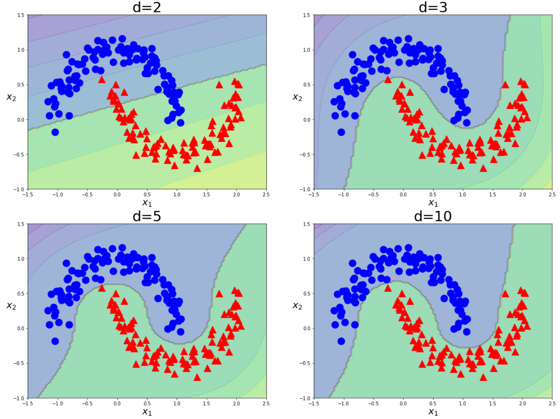
3次以降の写像はあまり変化がないことが読み取れる。