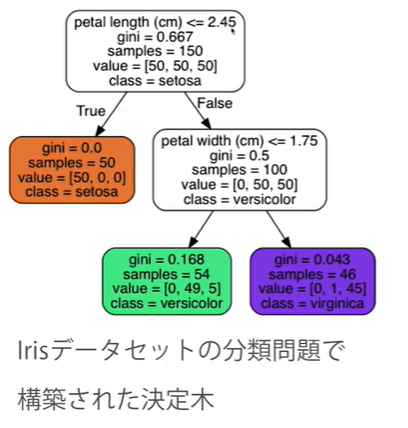
決定木とは？

決定木とは、ある簡単な基準に基づいてデータの分割を繰り返し、木のような構造を作り出すアルゴリズム。
分類・回帰問題の両方に適用可能
決定木は単体で使われることはすくない。(応用して、ランダムフォレストなど)

基準となる特徴量や閾値はどう決めるのか？

(分割前の不純度)-(分割後の不純度)
が最大になるように、分割の基準を決定する。

つまり、(分割後の不純度)が最小になるように分割を行う。

「不純度」とは、どれだけいろいろなクラスの観測値が混じりあっているかを表す指標。

分類問題の場合は、1つのノードに1つのクラスの観測値のみがあるのが理想(不純度=0)

不純度を表す関数

誤分類率(微分不可)
ジニ指数(微分可能)
交差エントロピー(微分可能)

が挙げられる。(sklearnのdefalutで設定されているのはジニ指数)

具体例

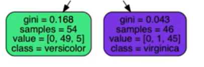
左：1 - (0/54)^2 - (49/54)^2 - (5/54)^2 = 0.168

右：1 - (0/46)^2 - (1/46)^2 - (45/46)^2 = 0.043

よって、全体の不純度は、
54/100 × 0.168 + 46/100 × 0.043 = 0.111(分割後の不純度)

決定木のメリットとデメリット

メリット

理解が容易
分類・回帰にいずれにも適用できる
あらゆる問題に広く適用できる
データの標準化 (正規化) やダミー変数の作成が不要

デメリット

分散が大きい(外れ値の影響を受けやすい)
過学習しやすい(ノンパラメトリックモデル)
予測面が滑らかでない

過学習を避けるには？

過学習を防止するためには、パラメータの調整が大切。

つまり、木の深さの上限(max-depth)や、1つのノードが最低持たなければならない観測値の数(min_samples_leaf)などを適切に設定する

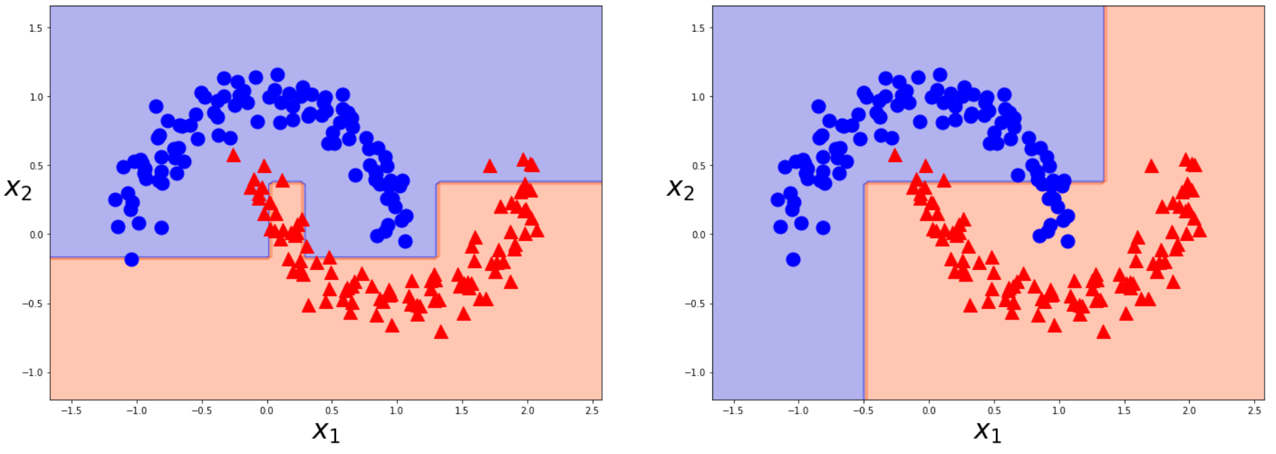
実験①(分類問題)

import numpy as np
import matplotlib.pyplot as plt
from sklearn.datasets import make_moons
from sklearn.model_selection import train_test_split

moons=make_moons(n_samples=200,noise=0.1,random_state=0)

X=moons[0]
y=moons[1]

X_train,X_test,y_train,y_test=train_test_split(X,y,random_state=0)

from sklearn.tree import DecisionTreeClassifier

tree_clf=DecisionTreeClassifier(min_samples_leaf=10).fit(X_train,y_train) #default上限なし
tree_clf_3=DecisionTreeClassifier(max_depth=3).fit(X_train,y_train)

print(tree_clf.score(X_test,y_test))
print(tree_clf_3.score(X_test,y_test))

from matplotlib.colors import ListedColormap

def plot_decision_boundary(model,X,y):
    _x1 = np.linspace(X[:,0].min()-0.5,X[:,0].max()+0.5,100)
    _x2 = np.linspace(X[:,1].min()-0.5,X[:,1].max()+0.5,100)
    x1,x2 = np.meshgrid(_x1,_x2)
    X_new=np.c_[x1.ravel(),x2.ravel()]
    y_pred=model.predict(X_new).reshape(x1.shape)
    custom_cmap=ListedColormap(["mediumblue","orangered"])
    plt.contourf(x1,x2,y_pred,cmap=custom_cmap,alpha=0.3)

def plot_dataset(X,y):
    plt.plot(X[:,0][y==0],X[:,1][y==0],"bo",ms=15)
    plt.plot(X[:,0][y==1],X[:,1][y==1],"r^",ms=15)
    plt.xlabel("$x_1$",fontsize=30)
    plt.ylabel("$x_2$",fontsize=30,rotation=0)

plt.figure(figsize=(24,8))
plt.subplot(121)
plot_decision_boundary(tree_clf,X,y)
plot_dataset(X,y)

plt.subplot(122)
plot_decision_boundary(tree_clf_3,X,y)
plot_dataset(X,y)

plt.show()

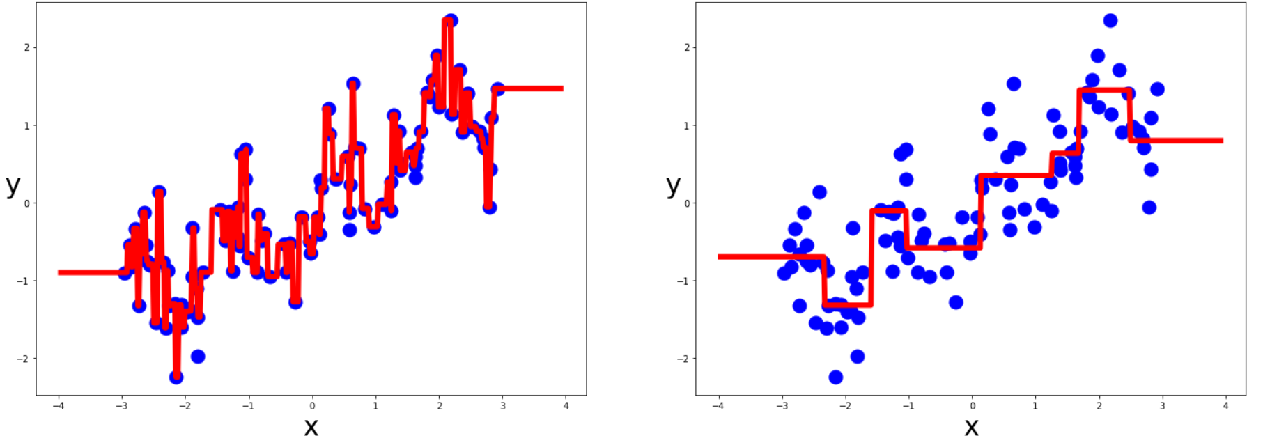
実験②(回帰問題)

import mglearn
from sklearn.tree import DecisionTreeRegressor

reg_X,reg_y=mglearn.datasets.make_wave(n_samples=100)

tree_reg=DecisionTreeRegressor().fit(reg_X,reg_y)
tree_reg_3=DecisionTreeRegressor(max_depth=3).fit(reg_X,reg_y)

def plot_regression_predicitons(model,X,y):
    x1 = np.linspace(X.min()-1,X.max()+1,500).reshape(-1,1)
    y_pred=model.predict(x1)
    plt.xlabel("x",fontsize=30)
    plt.ylabel("y",fontsize=30,rotation=0)
    plt.plot(X,y,"bo",ms=15)
    plt.plot(x1,y_pred,"r-",linewidth=6)

plt.figure(figsize=(24,8))

plt.subplot(121)
plot_regression_predicitons(tree_reg,reg_X,reg_y)

plt.subplot(122)
plot_regression_predicitons(tree_reg_3,reg_X,reg_y)

plt.show()