クラスター分析
-
クラスター…似ているもの同士の集まり。
-
クラスター分析とは、似ているデータ同士をグループ化する作業。
-
教師なし学習であるため、ラベル付けがなされていなデータをグループ化しなければならない。
→期待とは違ったグループ分けがなされることもある。 -
大きく**「階層的クラスタリング」と「非階層的クラスタリング」**に分けられる。
階層的クラスタリング
-
凝集型(下から上へ)…全てのデータについて、似ているデータ同士を逐次結び付けていく手法。
-
分割型(上から下へ)…全てのデータについて、似ていないもの同士を逐次分離させていく手法。
-
デンドログラムでクラスター形成の様子が見れる。
→理解が容易

似ている(似ていない)」はどう判断するのか?
- 多くの場合、類似度の測定には、ユークリッド距離が用いられる。つまり、2つのn次元データ
A:a=(a1,a2,.....,an)
B:b=(b1,b2,.....,bn)
の類似度は、以下のように決める。
d(A,B)=√{(a1-b1)^2+(a2-b2)^2+......+(an-bn)^2)}
クラスター間の距離
-
先の基準に基づいて似ているデータ同士を結びつけていくとクラスター(グループ)が形成される。
-
次の段階では、このクラスター(グループ)について似ているもの同士を結びつけなければいけない…
→クラスター(グループ)同士の距離はどう測るのか? -
クラスター間の距離の求め方はいくつかある。
1:最短距離法…2つのクラスターに含まれるデータの中で最も近いデータ同士の距離をクラスター間の距離とする。
2:最長距離法…2つのクラスターに含まれるデータの中で、最も遠いデータ同士の距離をクラスター間の距離とする。
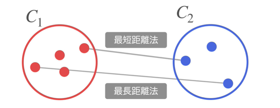
3:群平均法…2つのクラスター間に含まれる全てのデータ同士の距離の平均をクラスター間の距離とする。
4:重心法…2つのクラスターそれぞれの重心(平均のデータ)間の距離をクラスター間の距離とする。
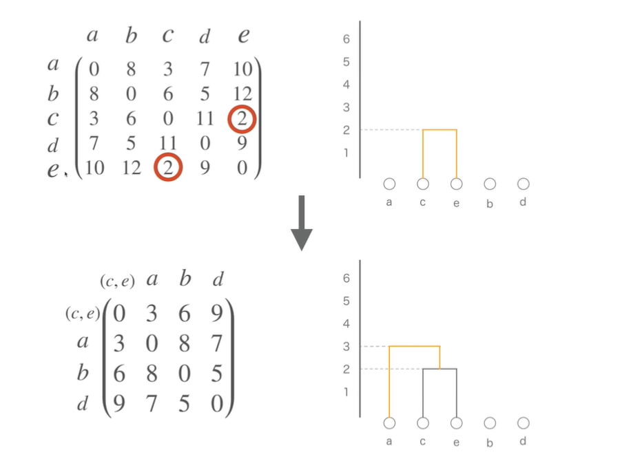
具体例(最短距離法)

非階層的クラスタリング
k-meansクラスタリングが最もポピュラー。手順は以下の通り。
1:ランダムにk個のクラスターの中心を決める。
2:全てのデータについて、1で定めたクラスターの中心のうち、最も近いものにデータを振り分け、k個のクラスターに分割する。
3:k個のクラスター重心(平均値)を求める。
4:3で求めた重心(平均値)を用いて、再度データを振り分ける。

実際にやってみた
以下のサイトからwebスクレイピングをして選手データを収集しました。
(スクレイピングの過程は省略)

データセット
import numpy as np
import pandas as pd
import matplotlib.pyplot as plt
import seaborn as sns
sns.set_style('whitegrid')

df = pd.read_csv('player_records.csv')
columns_list = ['年度', '所属球団', '登板', '勝利', '敗北', 'セーブ', 'H', 'HP',
                '完投', '完封勝', '無四球', '勝率', '打者', '投球回', '安打', '本塁打',
                '四球', '死球', '三振', '暴投', 'ボーク', '失点', '自責点', '防御率', '名前']
df = df.loc[:, columns_list]
df.head()

前処理
df.info()

# 防御率をobject型からfloat型へ
df['防御率'] = pd.to_numeric(df['防御率'], errors='coerce')
df.info()

# 欠損値削除
df.dropna(inplace=True)
from sklearn.preprocessing import StandardScaler
from sklearn.cluster import KMeans
from sklearn.metrics import silhouette_score, silhouette_samples
df = df[df['年度'] == 2019]

# 学習に使えないデータを削除する
data_df = df.drop(columns=['年度', '所属球団', '名前'])

# データの尺度を整える(クラスタリングには必須)
scaler = StandardScaler()
data_scaled = scaler.fit_transform(data_df)

data = np.array(data_df)
data_scaled = np.array(data_scaled)
教師なし学習(k-means法でモデル構築)
# エルボー法を用いてk_meansのkを決定する

distortions = []
for k in range(1, 11):
    kmeans = KMeans(n_clusters=k, n_init=10, max_iter=100)
    kmeans.fit(data_scaled)
    distortions.append(kmeans.inertia_)

fig = plt.figure(figsize=(12, 8))
plt.xticks(range(1, 11))
plt.plot(range(1, 11), distortions)

# 縦軸はクラスタ内平方和=どれだけ分類できてるか→小さいほうがよい
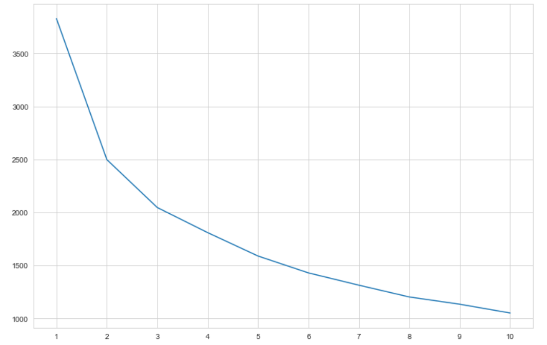
# 今回は3個に分類してみる
n_clusters = 3
kmeans = KMeans(n_clusters=n_clusters, n_init=10, max_iter=100)
kmeans.fit(data_scaled)
cluster_labels = kmeans.predict(data_scaled)
cluster_labels

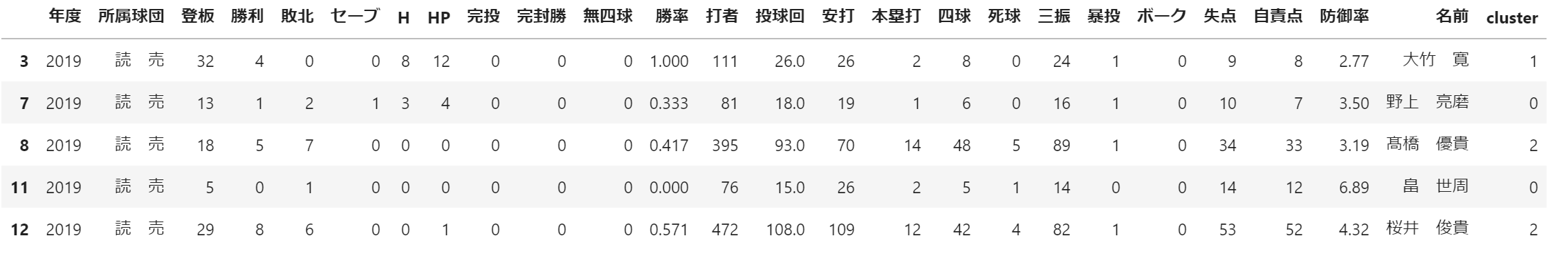
# カラムを途中省略せず、全部をみる方法
pd.set_option('display.max_columns', 30)
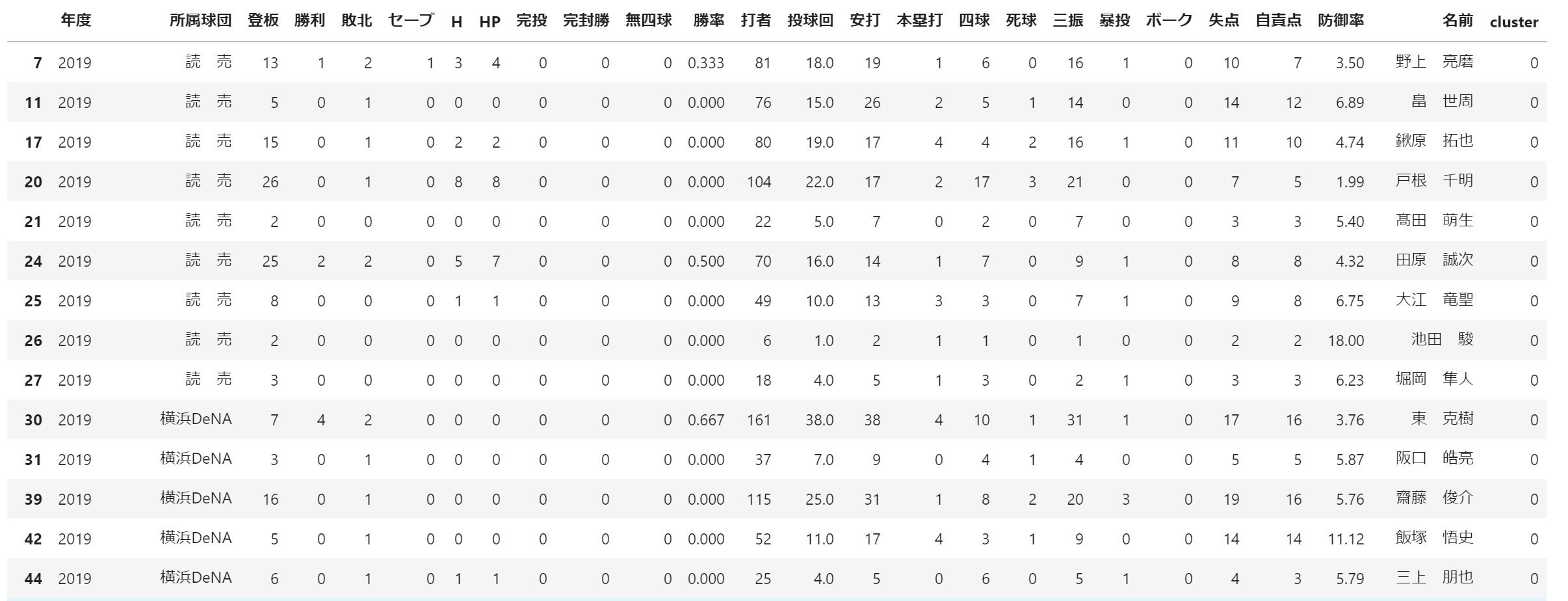
df['cluster'] = cluster_labels
df.head()
df[df['cluster'] == 0]
# 登板数多い、投球回と登板数が似ている。登板数少ない。
# 2軍中継ぎ投手?クローザー?
df[df['cluster'] == 1]
# 登板数多い、投球回と登板数が似ている。
# 一軍クローザーor中継ぎ

df[df['cluster'] == 2]
# 登板数<投球回が多い→先発投手?

# どのくらいの精度でクラスタリングできているか?

silhouette_avg = silhouette_score(data_scaled, cluster_labels)

silhouette_scores = silhouette_samples(data_scaled,
                                       cluster_labels,
                                       metric='euclidean')

colorlist = ['#87cefa', '#3cb371', '#ffa500', '#dc143c',
             '#ba55d3', '#a9a9a9', '#d8bfd8']

fig = plt.figure(figsize=(12, 8))
ax = fig.add_subplot(1, 1, 1)

y_lower = 0

for i in range(n_clusters):
    ith_cluster_silhouette_values = silhouette_scores[cluster_labels == i]
    ith_cluster_silhouette_values.sort()
    y_upper = y_lower + ith_cluster_silhouette_values.shape[0]

    color = colorlist[i]
    ax.fill_betweenx(np.arange(y_lower, y_upper), 0,
                     ith_cluster_silhouette_values,
                     facecolor=color, edgecolor=color)

    y_lower = y_upper

ax.set_xlabel('silhouette score')

# The vertical line for average silhouette score of all the values
ax.axvline(x=silhouette_avg, color='red', ls='--')

# 赤い線を超えてるほどよい
# 長方形程よい
