はじめに
本ブログは、プログラミングスクールでデータ分析の講座を約3ヶ月間勉強した後、そのカリキュラムの一環として受講修了のために公開しています。
今回は、メジャーリーグで大活躍中の大谷翔平選手の打席結果を予測するモデルの作成を行いました。
モデル作成の概要
今回のモデル作成では、大谷選手の打席結果についてアウトかヒットかを予測することを目的としました。打率やHR数など、シーズン単位の打撃成績の予測をする場合、メジャーリーグでプレーしたシーズンの数がまだ多くないことや、コロナ禍での短縮シーズンや怪我で欠場の多かったシーズンが外れ値となってしまう可能性が高いと考え、各打席での結果を予測するモデルを作成することとしました。
データはPythonのライブラリpybaseballを用いて、2021年のシーズン開幕から2024年の6月末を対象期間として取得しました。また、PythonのバージョンはPython3.10.12、実行環境はGoogle Colaboratoryです。
データ分析とモデル作成
データの取得と加工
以下のようにしてpybaseballのインストールとデータの取得を行いました。pb.playerid_lookupによって選手のIDを取得し、そのIDと期間を設定してpb.statcast_batterによってデータを取得します。
# pybaseballのインストール
!pip install pybaseball
import pybaseball as pb

# 大谷翔平のデータを取得
ohtani_info = pb.playerid_lookup('Ohtani', 'Shohei')

# バッティングのデータを取得
player_id = ohtani_info.iloc[0,2] # player_id = 660271
start_date = '2021-03-20'
end_date = '2024-06-30'
ohtani_data = pb.statcast_batter(start_date, end_date, player_id)
ohtani_data.head()
# 実行結果
	pitch_type	game_date	release_speed	release_pos_x	release_pos_z	player_name	batter	pitcher	events	description	...	post_home_score	post_bat_score	post_fld_score	if_fielding_alignment	of_fielding_alignment	spin_axis	delta_home_win_exp	delta_run_exp	bat_speed	swing_length
0	ST	2024-06-30	82.2	-1.77	6.07	Ohtani, Shohei	660271	702352	strikeout	swinging_strike	...	9	1	9	Strategic	Standard	61.0	0.003	-0.214	79.230797	8.69843
1	FF	2024-06-30	94.6	-1.96	5.96	Ohtani, Shohei	660271	702352	NaN	swinging_strike	...	9	1	9	Standard	Standard	236.0	0.000	-0.075	71.824988	6.41213
2	SI	2024-06-30	94.6	-1.95	6.04	Ohtani, Shohei	660271	702352	NaN	swinging_strike	...	9	1	9	Standard	Standard	238.0	0.000	-0.052	79.314620	7.71748
3	FF	2024-06-30	95.0	-1.94	6.05	Ohtani, Shohei	660271	702352	strikeout	swinging_strike	...	3	0	3	Standard	Standard	239.0	0.028	-0.291	74.372852	6.72873
4	CH	2024-06-30	88.7	-1.63	6.07	Ohtani, Shohei	660271	702352	NaN	blocked_ball	...	3	0	3	Standard	Standard	225.0	0.000	0.051	NaN	NaN
5 rows × 94 columns
取得したデータには、打者に対して投じられたすべての球ごとに94のデータ項目が含まれており、その一覧は以下のサイトで確認することができます。
# データ項目の一覧
print(ohtani_data.columns)
# 実行結果
Index(['pitch_type', 'game_date', 'release_speed', 'release_pos_x',
       'release_pos_z', 'player_name', 'batter', 'pitcher', 'events',
       'description', 'spin_dir', 'spin_rate_deprecated',
       'break_angle_deprecated', 'break_length_deprecated', 'zone', 'des',
       'game_type', 'stand', 'p_throws', 'home_team', 'away_team', 'type',
       'hit_location', 'bb_type', 'balls', 'strikes', 'game_year', 'pfx_x',
       'pfx_z', 'plate_x', 'plate_z', 'on_3b', 'on_2b', 'on_1b',
       'outs_when_up', 'inning', 'inning_topbot', 'hc_x', 'hc_y',
       'tfs_deprecated', 'tfs_zulu_deprecated', 'fielder_2', 'umpire', 'sv_id',
       'vx0', 'vy0', 'vz0', 'ax', 'ay', 'az', 'sz_top', 'sz_bot',
       'hit_distance_sc', 'launch_speed', 'launch_angle', 'effective_speed',
       'release_spin_rate', 'release_extension', 'game_pk', 'pitcher.1',
       'fielder_2.1', 'fielder_3', 'fielder_4', 'fielder_5', 'fielder_6',
       'fielder_7', 'fielder_8', 'fielder_9', 'release_pos_y',
       'estimated_ba_using_speedangle', 'estimated_woba_using_speedangle',
       'woba_value', 'woba_denom', 'babip_value', 'iso_value',
       'launch_speed_angle', 'at_bat_number', 'pitch_number', 'pitch_name',
       'home_score', 'away_score', 'bat_score', 'fld_score', 'post_away_score',
       'post_home_score', 'post_bat_score', 'post_fld_score',
       'if_fielding_alignment', 'of_fielding_alignment', 'spin_axis',
       'delta_home_win_exp', 'delta_run_exp', 'bat_speed', 'swing_length'],
      dtype='object')
上記データ項目のうち、打席の結果はeventsという項目に記載されます。
# 打席結果の一覧
ohtani_data['events'].value_counts()
# 実行結果
events
field_out                    757
strikeout                    588
single                       292
walk                         261
home_run                     156
double                       104
force_out                     42
grounded_into_double_play     29
triple                        27
hit_by_pitch                  14
field_error                   13
sac_fly                       11
catcher_interf                 7
fielders_choice                5
strikeout_double_play          2
double_play                    2
fielders_choice_out            1
pickoff_3b                     1
Name: count, dtype: int64
今回はアウトかヒットかの予測を行うため、以下のようにして新しくresultsというデータ項目を作り、打席結果がアウトなら0、ヒットなら1とします。
※今回は四死球などのアウトかヒットのいずれかでもなく打数に含まれない結果は除き、本来アウトになるはずであったfielders_choiceなどはアウトとして分類しています。また、今回は打席結果の予測であるため、結果が出ていない投球データ(例:ファールになったときの投球データ)は除いています。
# 打席結果の分類
def categorize_events(x):
  if x in ['field_out', 'strikeout', 'force_out', 'grounded_into_double_play', 'sac_fly',
             'fielders_choice', 'strikeout_double_play', 'double_play', 'fielders_choice_out']:
    return 0 # アウト
  elif x in ['single', 'double', 'triple', 'home_run']:
    return 1 # ヒット
  else:
    return None

ohtani_data['results'] = ohtani_data['events'].apply(lambda x: categorize_events(x))
ohtani_data = ohtani_data.dropna(subset=['results'])
更に、ランナーがいる場合はその選手のIDが記載されているため、ランナーがいる場合には1、いない場合には0となるようにデータを加工します。
# ランナーの有無を表示
ohtani_data[['on_1b', 'on_2b', 'on_3b']] = ohtani_data[['on_1b', 'on_2b', 'on_3b']].applymap(
    lambda x: 1 if pd.notna(x) else 0)
以下より、アウトかセーフで分類した打席結果と、主要なデータ項目の関係性を可視化します。
データの可視化
まずは球種や球速、コースと打席結果の関係性を図示します。
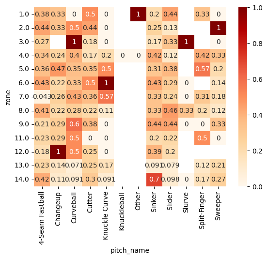
# 球種と打席結果の関係
import pandas as pd
import seaborn as sns

sns.heatmap(pd.crosstab(ohtani_data['pitch_name'], ohtani_data['results'], normalize='index'),
            annot=True, fmt='g', cmap='OrRd')
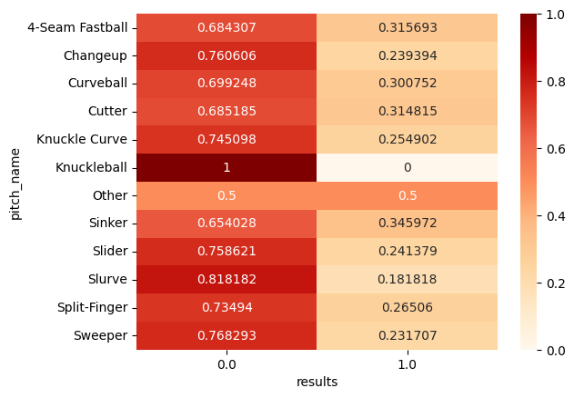
スライダー系、スプリット、チェンジアップ、ナックルカーブでアウトの割合が高くなっています。
# 球速と打席結果の関係
import matplotlib.pyplot as plt
import seaborn as sns

plt.figure(figsize=(4,4))
sns.boxplot(x='results', y='effective_speed', data=ohtani_data)
plt.show()
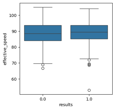
球速については打席結果にあまり影響を与えていないようです。
# コース(zone)と打席結果の関係
import pandas as pd
import seaborn as sns

sns.heatmap(pd.crosstab(ohtani_data['zone'], ohtani_data['results'], normalize='index'),
            annot=True, fmt='g', cmap='OrRd')
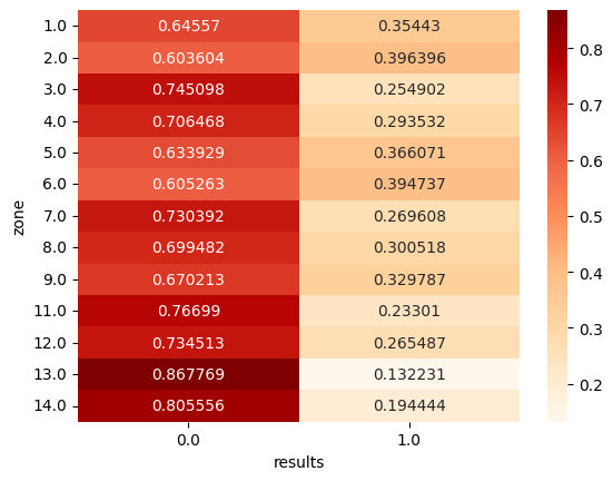
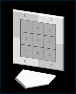
コースは下の図のようにストライクゾーンを9分割、ボールゾーンを4分割して数字を割り当てています。ボール球(特に低めの13, 14)や、左バッターにとってのインハイ(3)、アウトロー(7)でのアウトの割合が高くなっています。
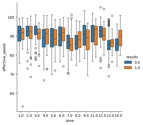
# 球速・コースと打席結果の関係
import matplotlib.pyplot as plt
import seaborn as sns

sns.catplot(x='zone', y='effective_speed', hue='results', data=ohtani_data,
            kind='box')
plt.show()
# 球種・コース(zone)とヒットの割合
import pandas as pd
import seaborn as sns

sns.heatmap(pd.pivot_table(ohtani_data, index='zone', columns='pitch_name', values='results',
               aggfunc='mean'), annot=True, cmap='OrRd')
アウトの割合が高いコースでも、球速や球種によってはヒットの割合が高くなっています。例えば、低めのボール球では球速が速いフォーシームやカットボールでヒットの割合が高く、インハイやアウトローでは球速が遅いカーブなどでヒットの割合が高くなっています。
次に、イニング、アウトカウント、打席内での投球数、ストライク・ボールのカウントとの関係性を図示します。
# イニング・アウトカウントとヒットの割合
import pandas as pd
import seaborn as sns

sns.heatmap(pd.pivot_table(ohtani_data, index='inning', columns='outs_when_up', values='results',
               aggfunc='mean'), annot=True, cmap='OrRd')
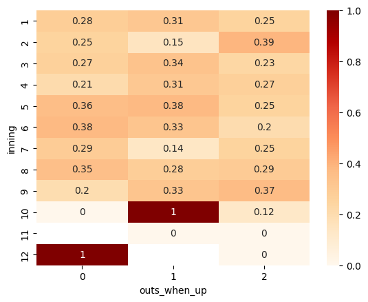
試合中盤のイニングや、2アウトになるまでのヒットの割合が他と比べて高くなっています。
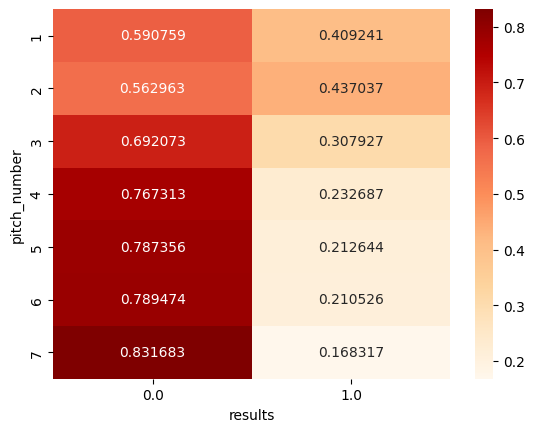
# 投球数と打席結果の関係
import pandas as pd
import seaborn as sns

pitch_number = ohtani_data[ohtani_data['pitch_number']<=7]
sns.heatmap(pd.crosstab(pitch_number['pitch_number'], pitch_number['results'], normalize='index'),
            annot=True, fmt='g', cmap='OrRd')
# 投球数・カウントと打席結果の関係
import pandas as pd
import seaborn as sns

pitch_number = ohtani_data[ohtani_data['pitch_number']<=7]
sns.heatmap(pd.crosstab(
    index=[pitch_number['pitch_number'], pitch_number['balls'], pitch_number['strikes']],
    columns=pitch_number['results'], normalize='index'), annot=True, fmt='g', cmap='OrRd')
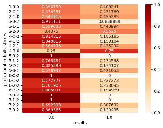
投球数については、データの数の少なかった8球目以降を除いた、7球目までに打席が終了した場合を抽出しています。比較的早い段階で2ストライクとなった場合には3, 4球目でのアウトの割合が高くなっていますが、そのような状況になる前の1, 2球目でのヒットの割合が高くなっています。
次にランナーの状況と打席結果の関係です。
# ランナーの状況と打席結果の関係
import seaborn as sns

sns.heatmap(pd.crosstab(
    index=[ohtani_data['on_1b'], ohtani_data['on_2b'], ohtani_data['on_3b']], columns=ohtani_data['results'],
    normalize='index'), annot=True, fmt='g', cmap='OrRd')
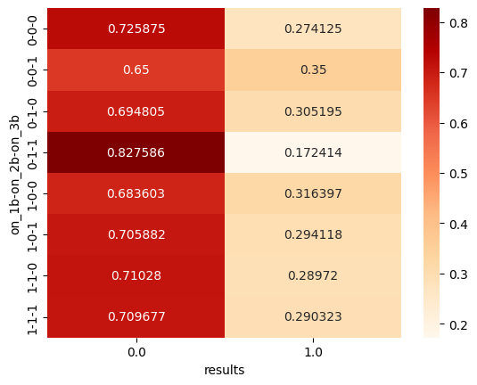
ランナー3塁のときが最もヒットの割合が高く、2, 3塁のとき最もヒットの割合が低なっています。
# ランナーの状況・アウトカウントとヒットの割合
import pandas as pd
import seaborn as sns

sns.heatmap(pd.pivot_table(ohtani_data, index=['on_1b', 'on_2b', 'on_3b'], columns='outs_when_up',
                           values='results', aggfunc='mean'), annot=True, cmap='OrRd')

また、アウトカウントと合わせると、フォースアウトが発生し得る状況ではアウトの割合が高くなっています。
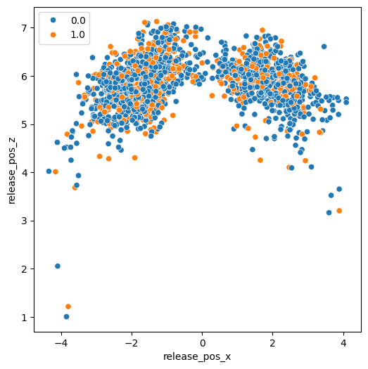
最後に、投手のリリースポイント(打者から見た位置)や変化量、回転数と打席結果の関係です。
# リリースポイントと打席結果の関係
import seaborn as sns
import matplotlib.pyplot as plt

plt.figure(figsize=(6,6))
sns.scatterplot(data=ohtani_data, x='release_pos_x', y='release_pos_z', hue='results')
plt.legend(loc='upper left')
plt.show()
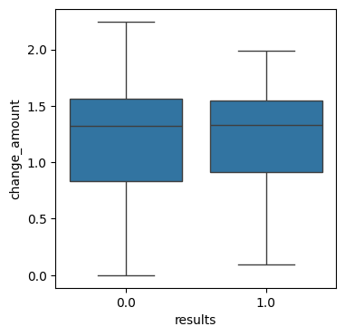
# ボールの変化量と打席結果の関係
import matplotlib.pyplot as plt
import seaborn as sns
import numpy as np

ohtani_data['change_amount'] = np.sqrt(ohtani_data['pfx_x']**2+ohtani_data['pfx_z']**2)
plt.figure(figsize=(4,4))
sns.boxplot(x='results', y='change_amount', data=ohtani_data)
plt.show()
# 回転数と打席結果の関係
import matplotlib.pyplot as plt
import seaborn as sns

plt.figure(figsize=(4,4))
sns.boxplot(x='results', y='release_spin_rate', data=ohtani_data)
plt.show()
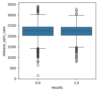
これらのデータ項目は打席結果とあまり関係しないことがわかりました。
予測モデルの作成
以上までの結果から、予測に用いるデータ項目を選択し、訓練データと検証データに分割しました。なお、p_throwsとpitch_nameはそれぞれLやR、球種名で記載されているため、One-hot encodingを行いました。
import pybaseball as pb
import pandas as pd
import numpy as np
from sklearn.model_selection import train_test_split

player_id = 660271
start_date = '2021-03-20'
end_date = '2024-06-30'
ohtani_data = pb.statcast_batter(start_date, end_date, player_id)

# 打席結果の分類(予測する項目)
def categorize_events(x):
  if x in ['field_out', 'strikeout', 'force_out', 'grounded_into_double_play', 'sac_fly',
           'fielders_choice', 'strikeout_double_play', 'double_play', 'fielders_choice_out']:
    return 0 # アウト
  elif x in ['single', 'double', 'triple', 'home_run']:
    return 1 # ヒット
  else:
    return None

ohtani_data['results'] = ohtani_data['events'].apply(lambda x: categorize_events(x))
ohtani_data = ohtani_data.dropna(subset=['results'])

# ランナーの有無を表示
ohtani_data[['on_1b', 'on_2b', 'on_3b']] = ohtani_data[['on_1b', 'on_2b', 'on_3b']].applymap(
    lambda x: 1 if pd.notna(x) else 0)

# 予測に用いるデータ項目を選択
features = [
    'zone', 'p_throws', 'balls', 'strikes', 'on_1b', 'on_2b', 'on_3b', 'outs_when_up', 'inning',
    'effective_speed', 'pitch_number', 'pitch_name', 'results'
    ]
sel_data = ohtani_data[features]

# One-hot encoding
sel_data = pd.get_dummies(sel_data, columns=['p_throws', 'pitch_name'])
sel_data = sel_data.dropna()

# 訓練データと検証データの準備
X = sel_data.drop(columns=['results'])
y = sel_data['results']
X_train, X_test, y_train, y_test = train_test_split(X, y, test_size=0.2, random_state=0)

# データ項目の詳細
X.info()
# 実行結果
 0   zone                        1960 non-null   float64
 1   balls                       1960 non-null   int64
 2   strikes                     1960 non-null   int64
 3   on_1b                       1960 non-null   int64
 4   on_2b                       1960 non-null   int64
 5   on_3b                       1960 non-null   int64
 6   outs_when_up                1960 non-null   int64
 7   inning                      1960 non-null   int64
 8   effective_speed             1960 non-null   float64
 9   pitch_number                1960 non-null   int64
 10  p_throws_L                  1960 non-null   bool
 11  p_throws_R                  1960 non-null   bool
 12  pitch_name_4-Seam Fastball  1960 non-null   bool
 13  pitch_name_Changeup         1960 non-null   bool
 14  pitch_name_Curveball        1960 non-null   bool
 15  pitch_name_Cutter           1960 non-null   bool
 16  pitch_name_Knuckle Curve    1960 non-null   bool
 17  pitch_name_Knuckleball      1960 non-null   bool
 18  pitch_name_Other            1960 non-null   bool
 19  pitch_name_Sinker           1960 non-null   bool
 20  pitch_name_Slider           1960 non-null   bool
 21  pitch_name_Slurve           1960 non-null   bool
 22  pitch_name_Split-Finger     1960 non-null   bool
 23  pitch_name_Sweeper          1960 non-null   bool
データ項目の数は24、データの総数は1960となりました。これらを用いて、ランダムフォレストとニューラルネットワークで予測を行いました。ランダムフォレストでは、ハイパーパラメータのmax_depthとn_estimatorsについて、accuracyが最大になるように適切な値を探索しました。
# ランダムフォレストによる予測
from sklearn.ensemble import RandomForestClassifier
from sklearn.metrics import classification_report

depth_list = [i for i in range(1, 21)]
estimators_list = [i for i in range(1, 101)]
max_score = 0

for max_depth in depth_list:
  for n_estimators in estimators_list:
    model = RandomForestClassifier(max_depth=max_depth, n_estimators=n_estimators,
                                   random_state=0)
    model.fit(X_train, y_train)
    score = model.score(X_test, y_test)
    if max_score < score:
      max_score = score
      best_max_depth = max_depth
      best_n_estimators = n_estimators

print(f'max_depth: {best_max_depth}, n_estimators: {best_n_estimators}, max_score: {max_score}')

model = RandomForestClassifier(max_depth=best_max_depth, n_estimators=best_n_estimators,
                               random_state=0)
model.fit(X_train, y_train)
y_pred = model.predict(X_test)
print(classification_report(y_test, y_pred))
# 実行結果
max_depth: 19, n_estimators: 14, max_score: 0.7244897959183674
              precision    recall  f1-score   support

         0.0       0.75      0.93      0.83       278
         1.0       0.57      0.23      0.32       114

    accuracy                           0.72       392
   macro avg       0.66      0.58      0.58       392
weighted avg       0.69      0.72      0.68       392
# ニューラルネットワークによる予測
import numpy as np
import tensorflow as tf
from sklearn.metrics import accuracy_score, classification_report
import random
import os

tf.random.set_seed(0)
np.random.seed(0)
random.seed(0)
os.environ['PYTHONHASHSEED'] = '0'

train_X, test_X = X_train.astype(float), X_test.astype(float)
train_y, test_y = y_train.values, y_test.values

model = tf.keras.models.Sequential([
    tf.keras.layers.Input((train_X.shape[1],)),
    tf.keras.layers.Dense(16, activation='relu'),
    tf.keras.layers.Dense(8, activation='relu'),
    tf.keras.layers.Dense(1, activation='sigmoid')])

model.compile(optimizer=tf.keras.optimizers.Adam(learning_rate=0.001),
              loss='binary_crossentropy',
              metrics=['binary_accuracy'])

model.fit(train_X, train_y, batch_size=16, epochs=200, verbose=False)

pred_test_y = model.predict(test_X)
pred_test_y_binary = np.where(pred_test_y>0.5, 1, 0)
print(f'test_score: {accuracy_score(test_y, pred_test_y_binary)}')
print(f'test_report: \n{classification_report(test_y, pred_test_y_binary)}')
# 実行結果
test_score: 0.7117346938775511
test_report:
              precision    recall  f1-score   support

         0.0       0.73      0.94      0.82       278
         1.0       0.51      0.16      0.24       114

    accuracy                           0.71       392
   macro avg       0.62      0.55      0.53       392
weighted avg       0.67      0.71      0.65       392
ランダムフォレストでaccuracyが0.72となり、ニューラルネットワークの結果をわずかに上回りました。
次に、予測モデルは上記と変更せずに、投手の左右でデータを分割して予測を行いました。
# 投手の左右でデータを分割(以下は左投手の場合)
sel_data_left = sel_data.query('p_throws_L==True')
X = sel_data_left.drop(columns=['results', 'p_throws_L', 'p_throws_R'])
y = sel_data_left['results']
X_train, X_test, y_train, y_test = train_test_split(X, y, test_size=0.2, random_state=0)
上記の処理によって訓練データ、検証データを用意し、それぞれ予測をした結果は以下の通りです。
# ランダムフォレスト・左投手
max_depth: 9, n_estimators: 8, max_score: 0.7744360902255639
              precision    recall  f1-score   support

         0.0       0.77      0.97      0.86        95
         1.0       0.79      0.29      0.42        38

    accuracy                           0.77       133
   macro avg       0.78      0.63      0.64       133
weighted avg       0.78      0.77      0.74       133

# ランダムフォレスト・右投手
max_depth: 7, n_estimators: 6, max_score: 0.7423076923076923
              precision    recall  f1-score   support

         0.0       0.77      0.93      0.84       187
         1.0       0.59      0.27      0.37        73

    accuracy                           0.74       260
   macro avg       0.68      0.60      0.61       260
weighted avg       0.72      0.74      0.71       260

# ニューラルネットワーク・左投手
test_score: 0.6917293233082706
test_report:
              precision    recall  f1-score   support

         0.0       0.72      0.93      0.81        95
         1.0       0.36      0.11      0.16        38

    accuracy                           0.69       133
   macro avg       0.54      0.52      0.49       133
weighted avg       0.62      0.69      0.63       133

# ニューラルネットワーク・右投手
test_score: 0.6807692307692308
test_report:
              precision    recall  f1-score   support

         0.0       0.77      0.79      0.78       187
         1.0       0.43      0.40      0.41        73

    accuracy                           0.68       260
   macro avg       0.60      0.59      0.60       260
weighted avg       0.67      0.68      0.68       260
ニューラルネットワークでのスコアの向上は見られませんでしたが、ランダムフォレストでは左右ともにスコアが向上しました。
今回のデータでは、アウト・ヒットの2つのクラスの数に差があるため、以下からはアンダーサンプリングやオーバーサンプリングによって訓練データの数を変更して、予測を行いました。なお、すべて前述の訓練データと検証データの準備と同様の処理を行った後にデータ数を変更しています。また、予測モデルは前述と同様のままです。
# RandomUnderSamplerによるアンダーサンプリング
from imblearn.under_sampling import RandomUnderSampler

rs = RandomUnderSampler(random_state=0)
X_train, y_train = rs.fit_resample(X_train, y_train)
# ランダムフォレスト
max_depth: 17, n_estimators: 2, max_score: 0.6811224489795918
              precision    recall  f1-score   support

         0.0       0.75      0.83      0.79       278
         1.0       0.44      0.32      0.37       114

    accuracy                           0.68       392
   macro avg       0.59      0.58      0.58       392
weighted avg       0.66      0.68      0.67       392

# ニューラルネットワーク
test_score: 0.6096938775510204
test_report:
              precision    recall  f1-score   support

         0.0       0.77      0.64      0.70       278
         1.0       0.38      0.54      0.45       114

    accuracy                           0.61       392
   macro avg       0.58      0.59      0.57       392
weighted avg       0.66      0.61      0.63       392
アンダーサンプリングではスコアの改善が見られず、特にニューラルネットワークではスコアが大きく下がってしまいました。
# ランダムフォレスト・左投手
max_depth: 2, n_estimators: 2, max_score: 0.7142857142857143
              precision    recall  f1-score   support

         0.0       0.81      0.78      0.80        95
         1.0       0.50      0.55      0.53        38

    accuracy                           0.71       133
   macro avg       0.66      0.67      0.66       133
weighted avg       0.72      0.71      0.72       133

# ランダムフォレスト・右投手
max_depth: 10, n_estimators: 79, max_score: 0.6730769230769231
              precision    recall  f1-score   support

         0.0       0.82      0.70      0.76       187
         1.0       0.44      0.60      0.51        73

    accuracy                           0.67       260
   macro avg       0.63      0.65      0.63       260
weighted avg       0.71      0.67      0.69       260

# ニューラルネットワーク・左投手
test_score: 0.631578947368421
test_report:
              precision    recall  f1-score   support

         0.0       0.83      0.61      0.70        95
         1.0       0.41      0.68      0.51        38

    accuracy                           0.63       133
   macro avg       0.62      0.65      0.61       133
weighted avg       0.71      0.63      0.65       133

# ニューラルネットワーク・右投手
test_score: 0.5884615384615385
test_report:
              precision    recall  f1-score   support

         0.0       0.78      0.59      0.67       187
         1.0       0.36      0.58      0.44        73

    accuracy                           0.59       260
   macro avg       0.57      0.58      0.56       260
weighted avg       0.66      0.59      0.61       260
投手の左右でデータを分割した場合にも、ニューラルネットワークではスコアの大幅な低下が見られ、アンダーサンプリングではスコアが改善しませんでした。
# RandomOverSamplerによるオーバーサンプリング
from imblearn.over_sampling import RandomOverSampler

ros = RandomOverSampler(random_state=0, sampling_strategy='minority')
X_train, y_train = ros.fit_resample(X_train, y_train)
# ランダムフォレスト
max_depth: 14, n_estimators: 29, max_score: 0.7040816326530612
              precision    recall  f1-score   support

         0.0       0.77      0.83      0.80       278
         1.0       0.49      0.40      0.44       114

    accuracy                           0.70       392
   macro avg       0.63      0.62      0.62       392
weighted avg       0.69      0.70      0.69       392

# ニューラルネットワーク
test_score: 0.6275510204081632
test_report:
              precision    recall  f1-score   support

         0.0       0.80      0.63      0.71       278
         1.0       0.41      0.61      0.49       114

    accuracy                           0.63       392
   macro avg       0.60      0.62      0.60       392
weighted avg       0.69      0.63      0.64       392
ランダムフォレストではスコアが0.7を超えましたが、ニューラルネットワークでの改善は見られませんでした。
# ランダムフォレスト・左投手
max_depth: 20, n_estimators: 44, max_score: 0.7669172932330827
              precision    recall  f1-score   support

         0.0       0.81      0.87      0.84        95
         1.0       0.61      0.50      0.55        38

    accuracy                           0.77       133
   macro avg       0.71      0.69      0.70       133
weighted avg       0.76      0.77      0.76       133

# ランダムフォレスト・右投手
max_depth: 10, n_estimators: 27, max_score: 0.7153846153846154
              precision    recall  f1-score   support

         0.0       0.82      0.77      0.80       187
         1.0       0.49      0.58      0.53        73

    accuracy                           0.72       260
   macro avg       0.66      0.67      0.66       260
weighted avg       0.73      0.72      0.72       260

# ニューラルネットワーク・左投手
test_score: 0.42857142857142855
test_report:
              precision    recall  f1-score   support

         0.0       0.74      0.31      0.43        95
         1.0       0.30      0.74      0.42        38

    accuracy                           0.43       133
   macro avg       0.52      0.52      0.43       133
weighted avg       0.62      0.43      0.43       133

# ニューラルネットワーク・右投手
test_score: 0.6269230769230769
test_report:
              precision    recall  f1-score   support

         0.0       0.78      0.67      0.72       187
         1.0       0.38      0.52      0.44        73

    accuracy                           0.63       260
   macro avg       0.58      0.59      0.58       260
weighted avg       0.67      0.63      0.64       260
ニューラルネットワークではアンダーサンプリングと同様に改善が見られませんでしたが、ランダムフォレストの左投手ではスコアが0.77まで向上しました。
最後に、SMOTE-ENNによってデータ数を変更して、予測を行いました。
# SMOTE-ENNによる処理
from imblearn.over_sampling import SMOTE
from imblearn.under_sampling import EditedNearestNeighbours
from imblearn.combine import SMOTEENN

sm_enn = SMOTEENN(
    smote=SMOTE(k_neighbors=2, random_state=0),
    enn=EditedNearestNeighbours(n_neighbors=3))
X_train, y_train = sm_enn.fit_resample(X_train, y_train)
# ランダムフォレスト
max_depth: 14, n_estimators: 51, max_score: 0.7168367346938775
              precision    recall  f1-score   support

         0.0       0.75      0.90      0.82       278
         1.0       0.53      0.26      0.35       114

    accuracy                           0.72       392
   macro avg       0.64      0.58      0.58       392
weighted avg       0.68      0.72      0.68       392

# ニューラルネットワーク
test_score: 0.6964285714285714
test_report:
              precision    recall  f1-score   support

         0.0       0.73      0.90      0.81       278
         1.0       0.45      0.20      0.28       114

    accuracy                           0.70       392
   macro avg       0.59      0.55      0.54       392
weighted avg       0.65      0.70      0.65       392
ランダムフォレスト、ニューラルネットワークともに0.7前後でした。
# ランダムフォレスト・左投手
max_depth: 19, n_estimators: 9, max_score: 0.7969924812030075
              precision    recall  f1-score   support

         0.0       0.85      0.87      0.86        95
         1.0       0.66      0.61      0.63        38

    accuracy                           0.80       133
   macro avg       0.75      0.74      0.75       133
weighted avg       0.79      0.80      0.79       133

# ランダムフォレスト・右投手
max_depth: 9, n_estimators: 46, max_score: 0.7384615384615385
              precision    recall  f1-score   support

         0.0       0.79      0.86      0.83       187
         1.0       0.54      0.42      0.48        73

    accuracy                           0.74       260
   macro avg       0.67      0.64      0.65       260
weighted avg       0.72      0.74      0.73       260

# ニューラルネットワーク・左投手
test_score: 0.6616541353383458
test_report:
              precision    recall  f1-score   support

         0.0       0.78      0.73      0.75        95
         1.0       0.42      0.50      0.46        38

    accuracy                           0.66       133
   macro avg       0.60      0.61      0.61       133
weighted avg       0.68      0.66      0.67       133

# ニューラルネットワーク・右投手
test_score: 0.7307692307692307
test_report:
              precision    recall  f1-score   support

         0.0       0.75      0.94      0.83       187
         1.0       0.56      0.21      0.30        73

    accuracy                           0.73       260
   macro avg       0.65      0.57      0.57       260
weighted avg       0.70      0.73      0.68       260
投手の左右で分割した場合、ランダムフォレストではスコアが高く、特に左投手では今回の検討の中では最高の約0.8となりました。
結果のまとめと考察
これまでの検討の結果、全体的にランダムフォレストによる予測で高いスコアを記録しました。また、データを投手の左右で分割したり、SMOTE-ENNで前処理を行うことによってスコアが改善しました。
# 主な結果(accuracy)

# ランダムフォレスト
全データ:0.724
左投手:0.774
右投手:0.742

# SMOTE-ENN・ランダムフォレスト
全データ:0.717
左投手:0.797
右投手:0.738
野球では、どれだけ良いバッターでも通算の打率としては3割台であり、アウトかヒットかで打席の結果を分類する場合にはクラス数の差が課題になると考えられます。今回の検討では、アンダーサンプリングでは予測精度が向上しませんでしたが、オーバーサンプリングやSMOTE-ENNを用いることで結果が良くなる傾向が見られたため、少数クラスに対して適切な処理を行うことが予測精度の向上に繋がることが示唆されました。
また、仮に今回の予測モデルを実際に活用する場合、例えばどのようなタイミングでどのようなピッチャーを投入し、どのようなボールを投げれば大谷選手を抑えることができるのか、データに基づいて決定するという場合が考えられます。投げるボールについては、実際に意図した通りに投げることができるかわからないですが、例えば左投手か右投手かという点は投げる前に確定している条件になります。そのため、前述の通り投手の左右でデータを分割した場合にはよりスコアの高いモデルとなっていることから、それらを活用することが得策と考えられます。また、予測結果がヒットになる場合にはそもそもその状況をなるべく避けた上で、アウトという予測結果に対して実際にアウトになることが重要となります。その点を考えると、アウトに対するPrecisionやヒットに対するRecallが高いということが予測モデルに求められるため、それらを指標にモデルの選定やハイパーパラメータの探索を行うことも有効な手段かもしれません。
最後に
今回は、pybaseballによって取得した野球の打撃データを活用して、打席の結果を予測するモデルの作成を行いました。pybaseballでは他にも投手の投球データの詳細など、多岐にわたるデータを取得することができます。また、近年は他のスポーツでもデータを活用して戦術を立てることが多くなっているため、今後も学んだことを活かしてスポーツに関するデータ分析や予測モデルの作成に取り組んでみたいと思います。