Deep Evidential Regression【4 Experiments】【論文 DeepL 翻訳】

この記事は自分用のメモみたいなものです.
ほぼ DeepL 翻訳でお送りします.
間違いがあれば指摘していだだけると嬉しいです.

翻訳元
Deep Evidential Regression
Author: Alexander Amini, Wilko Schwarting, Ava Soleimany, Daniela Rus

前: 【3 Evidential uncertainty for regression】
次: 【5 Related work】

4 Experiments

訳文

4.1 Predictive accuracy and uncertainty benchmarking

最初に, 一次元の三次回帰データセット上のベースラインに対する我々のアプローチの性能を定性的に比較する (図 3). [20, 28] に従って, $y = x^3 + \epsilon$, でモデルを学習する. ここで, $\epsilon \sim \mathcal{N} (0, 3)$ が $\pm 4$ 以内, 検定が $\pm 6$ 以内である. ベースライン法 (左), 正則化なしのエビデンス (中), 正則化ありのエビデンス (右) について, aleatoric uncertainty (A) と epistemic uncertainty (B) 推定を比較している. それぞれのベースライン法として Gaussian MLE [36] と Ensembling [28] を用いた. すべての aleatoric 手法 (A) は, 予想通り, 訓練分布内の不確実性を正確に捕捉する. Epistemic uncertainty (B) は OOD データ上の不確かさを捕捉する; 我々の提案するエビデンス法は不確かさを適切に推定し, サンプリングに依存せずに OOD データ上で成長する. この例の訓練の詳細と追加の実験は, S2.1 節に記載されている.

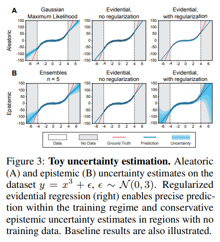
図 3 : トイデータセットの不確かさ推定. データセット $y = x 3 + \epsilon$, $\epsilon \sim \mathcal{N} (0, 3)$ の aleatoric uncertainty (A) と epistemic uncertainty (B) 推定. 正則化された evidential regression (右) は, 訓練領域内では正確な予測を可能にし, 訓練データのない領域では保守的な epistemic uncertainty の推定を可能にする. ベースラインの結果も示されている.

さらに, [20, 28, 9] で使用された実世界のデータセット上での NN 予測不確かさ推定のためのベースライン手法と我々のアプローチを比較する. 我々は, モデルアンサンブル [28] およびドロップアウト [9] の結果に対して, 提案した evidential regression 手法を, 二乗平均誤差 (RMSE), 負の対数尤度 (NLL), および推論速度に基づいて評価する. 表 1 は, 競合するアプローチとは異なり, evidential regression の損失関数は明示的に精度を最適化していないにもかかわらず, RMSE に関しては競争力を維持しており, NLL と速度に関してはすべてのデータセットでトップパフォーマーであることを示している. 2 つのベースライン手法を最大限に活用するために, サンプル推論を並列化した $(n = 5)$. ドロップアウトでは, サンプリングされたマスクの追加の乗算が必要となり, アンサンブルに比べて推論が若干遅くなるが, エビデンスではフォワードパスとネットワークが 1 回で済む. 表 1 のトレーニングの詳細は, S2.2 にある.

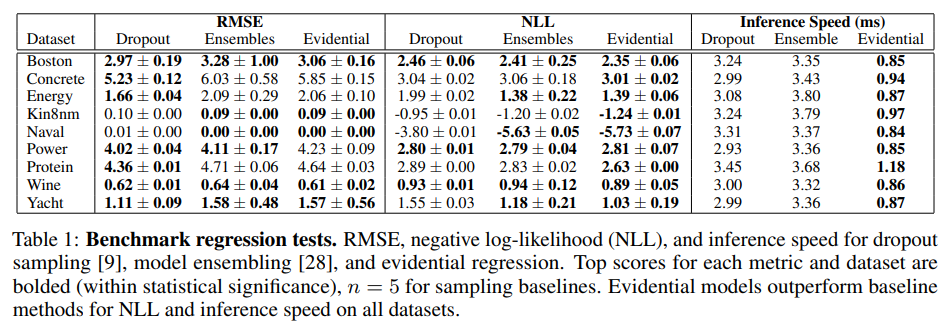
表 1: ベンチマーク回帰検定. ドロップアウトサンプリング [9], モデルアンサンブル[28], および evidential regression の RMSE, 負の対数尤度 (NLL), および推論速度. 各メトリックとデータセットのトップスコアは太字 (統計的有意性の範囲内), サンプリングのベースラインについては $n = 5$. エビデンスモデルは, すべてのデータセットにおいて, NLL と推論速度の面でベースライン手法よりも優れている.

4.2 Monocular depth estimation

ベンチマーク比較の結果を確立した後, このサブセクションでは, 複雑で高次元の課題である深度推定に拡張することで, 我々のエビデンス学習アプローチのスケーラビリティを実証する. 単眼的なエンドツーエンドの奥行き推定はコンピュータビジョンの中心的な問題であり, シーンの RGB 画像から直接奥行きの表現を学習する. これは、ターゲット $y$ が非常に高次元であり, 各ピクセルでの予測が必要となるため, 難しい学習タスクである.

我々の学習データは, NYU Depth v2 データセット [35] からの 27k 以上の RGB-to-Depth, $H \times W$ の屋内シーン (キッチン, 寝室など) の画像ペアから構成されている. 推論のために U-Net スタイルの NN [41] を訓練し, シーンの不連続なテストセット (3) でテストを行う. 最終層は, バニラ回帰, ドロップアウト, アンサンブルの場合, 単一の $H \times W$ 活性化マップを出力する. Spatial dropout uncertainty sampling [2, 45] がドロップアウトの実装に使用される. Evidential regression は, $(\gamma, \upsilon, \alpha, \beta)$ に対応するこれらの出力マップのうち 4 つを, Sec.3.3 に従った制約で出力する.

我々は, 未知のテストデータ上でのモデルの精度と予測 epistemic uncertainty の観点から評価を行う. 図 4A は, ランダムに選ばれた 2 つのテスト画像について, 予測された深さ, グラウンドトゥルースからの絶対誤差, 予測エントロピーを可視化したものである. 理想的には, 強い epistemic uncertainty の尺度は, 予測のエラーを捕捉するだろう (すなわち, モデルがエラーを起こしている場所に大体対応している). ドロップアウトやアンサンブルと比較して, エビデンスモデリングは, 信頼度の明確で局所的な予測を提供しながら, 深さ方向の誤差を捕捉する. 一般的に, ドロップアウトは存在する不確実性の量を大幅に過小評価するが, アンサンブルリングは不確実性を過大評価することがある. 図 4B は, 特定のしきい値以上の不確実性を持つピクセルが除去されたときの各モデルの性能を示している. 信頼度が高くなるにつれて誤差が着実に減少しているため, 根拠のあるモデルは強力な性能を示している.

図 4C は, さらに, 我々の不確かさ推定値の較正を評価している. 較正曲線は [27] に従って計算され, 理想的には $y = x$ に従い, 例えば, ターゲットが約 90% の信頼区間に約 90% の時間で落ちることを表す. ここでも, 信頼度の低いシナリオを考慮した場合, ドロップアウトが信頼度を過大評価していることがわかる (校正誤差: 0.126). アンサンブルリングは, より良い較正誤差 (0.048) を示したが, 提案されたエビデンス手法 (0.033) よりも優れている.

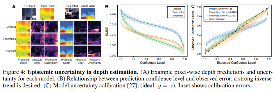
Figure 4: Epistemic uncertainty in depth estimation. (A) Example pixel-wise depth predictions and uncertainty for each model. (B) Relationship between prediction confidence level and observed error; a strong inverse trend is desired. (C) Model uncertainty calibration [27]; (ideal: y = x). Inset shows calibration errors.

epistemic uncertainty の実験に加えて, ガウス型 MLE 学習との比較を行いながら, aleatoric uncertainty の推定値を評価する. エビデンスモデルはデータを高次のガウス分布に適合させるので, ([42, 18] でも示されているように) 正確に不確かさを学習できると期待される. したがって, 我々は, これらの aleatoric な結果を S3.4 節で提示し, 結果の残りの部分は, 分布外 (OOD) と逆に摂動したサンプルの文脈での epistemic uncertainty 推定のより困難な課題を評価することに焦点を当てている.

4.3 Out-of distribution testing

不確実性推定の主な用途は, モデルが分布から外れた (OOD) テストサンプルに直面したとき, またはモデルの出力が信頼できないときに理解することである. このサブセクションでは, 多様な屋外走行の OOD データセットであるApolloScape [21] からの画像をテストすることで, OOD データ上で増加した epistemic uncertainty を捕捉するためのエビデンスモデルの能力を調査する. ここで重要なことは, 分類における事前ネットワーク [32, 33] のような関連手法は, 高い不確実性のインスタンスを監視するために, 訓練中に明示的に OOD データを必要とすることである.
我々の実証的手法は, ベイズ型 NN のようにこの制限を持たず, 訓練中の分布 (ID) データのみを見る.

各手法について, ID と OOD のテストセットを与え, 各テスト画像について平均予測エントロピーを記録する. 図 5A は, 各手法とテストセットについてのエントロピーの累積密度関数 (CDF) を示している. エントロピーの CDF には, OOD データ上のエビデンスモデルに対して明確な正のシフトが見られ, 手法間で競合している. 図 5B は, これらのエントロピー分布を四分位間ボックスプロットとしてまとめたもので, OOD データ上の不確実性分布に明確な分離があることを示している. 図 5C ではエビデンスモデルからの分布に焦点を当て, 図 5D ではサンプル予測 (ID と OOD) を提供している. これらの結果は, OOD データ上での訓練なしで, エビデンスモデルが, epistemic uncertainty 推定のベースラインと同等に, OOD データ上で増加した不確実性を捕捉していることを示している.

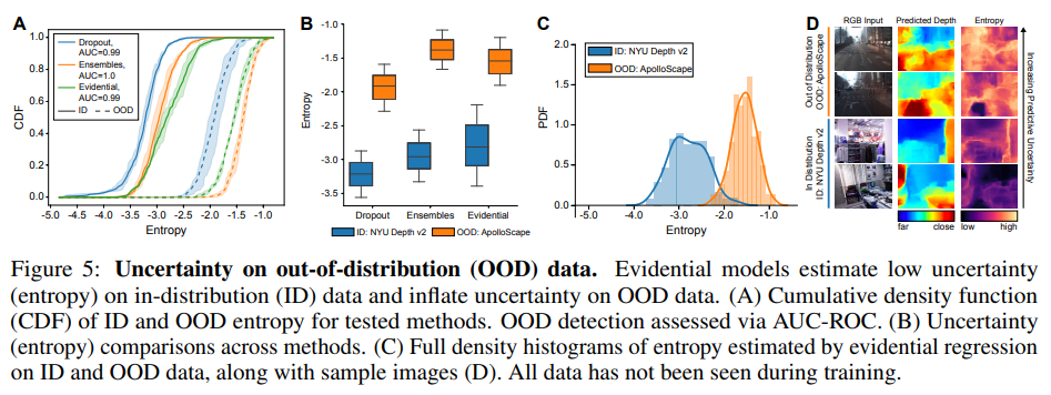
図 5: 分布外 (OOD) データの不確実性. 証拠モデルは, 分布内 (ID) データの低い不確実性 (エントロピー) を推定し, 分布外 (OOD) データの不確実性を増大させる. (A) テストされた手法の ID と OOD のエントロピーの累積密度関数 (CDF). OOD 検出は AUC-ROC で評価. (B) 手法間の不確かさ (エントロピー) の比較. (C) ID と OOD データ上でのevidential regression によって推定されたエントロピーの完全密度ヒストグラムとサンプル画像 (D). すべてのデータは訓練中には見られていない。

4.3.1 Robustness to adversarial samples

次に, OOD 検出の極端なケースとして, 入力が予測値に誤差を与えるために敵対的に摂動される場合を検討する. 我々は, 高速勾配符号法 (FGSM) [16] を用いて, ノイズのスケールを増加させながら, テストセットに対する敵対的摂動を計算する. この実験の目的は, 最先端の敵対的攻撃に対する防御策を提案することではなく, むしろ, 敵対的摂動が行われたサンプルの予測の不確かさの増大をエビデンスモデルが正確に捉えていることを実証することであることに注意する必要がある. 図 6A は, 敵対的なノイズが加わると, すべての手法の絶対誤差が増加することを確認している. また, 図 6B では, predictive uncertainty の推定値にノイズが正の効果を示している. さらに, エントロピー CDF は, 入力サンプルのノイズが増加するにつれて, より高い不確かさに向かって着実にシフトしていることが観察される( 図6C).

敵対的摂動に対するエビデンス不確実性のロバスト性は, 図 6D でより詳細に視覚化される. これは, 入力画像をより多くのノイズ (左から右) で摂動させたときの予測深度, エラー, および推定ピクセル単位の不確実性を示している. predictive uncertainty は, ノイズの増加とともに着実に増加するだけでなく, 画像全体の不確かさの空間的な濃度もまた, 誤差と緊密に対応している.

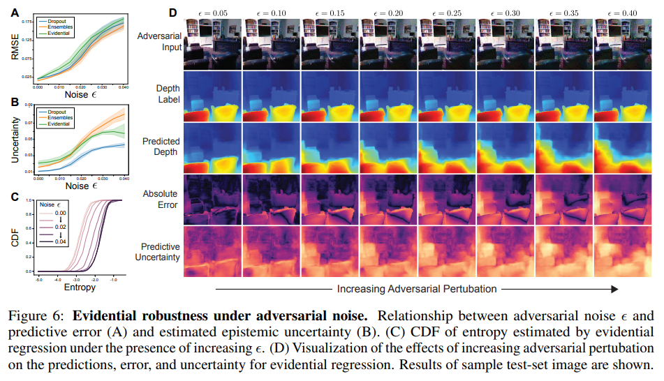
図 6: 敵対的ノイズの下でのエビデンスロバスト性. 敵対的ノイズと予測誤差 (A) および epistemic uncertainty (B) との関係. (D) evidential regression の予測, 誤差, 不確実性に対する敵対的摂動の増加の効果の可視化. サンプルテストセット画像の結果を示す.

原文

4.1 Predictive accuracy and uncertainty benchmarking

We first qualitatively compare the performance of our approach against a set of baselines on a onedimensional cubic regression dataset (Fig. 3). Following [20, 28], we train models on $y = x^3 + \epsilon$, where $\epsilon \sim \mathcal{N} (0, 3)$ within $\pm 4$ and test within $\pm 6$. We compare aleatoric (A) and epistemic (B) uncertainty estimation for baseline methods (left), evidence without regularization (middle), and with regularization (right). Gaussian MLE [36] and Ensembling [28] are used as respective baseline methods. All aleatoric methods (A) accurately capture uncertainty within the training distribution, as expected. Epistemic uncertainty (B) captures uncertainty on OOD data; our proposed evidential method estimates uncertainty appropriately and grows on OOD data, without dependence on sampling. Training details and additional experiments for this example are available in Sec. S2.1.

Figure 3: Toy uncertainty estimation. Aleatoric (A) and epistemic (B) uncertainty estimates on the dataset $y = x 3 + \epsilon$, $\epsilon \sim \mathcal{N} (0, 3)$. Regularized evidential regression (right) enables precise prediction within the training regime and conservative epistemic uncertainty estimates in regions with no training data. Baseline results are also illustrated.

Additionally, we compare our approach to baseline methods for NN predictive uncertainty estimation on real world datasets used in [20, 28, 9]. We evaluate our proposed evidential regression method against results presented for model ensembles [28] and dropout [9] based on root mean squared error (RMSE), negative log-likelihood (NLL), and inference speed. Table 1 indicates that even though, unlike the competing approaches, the loss function for evidential regression does not explicitly optimize accuracy, it remains competitive with respect to RMSE while being the top performer on all datasets for NLL and speed. To give the two baseline methods maximum advantage, we parallelize their sampled inference $(n = 5)$. Dropout requires additional multiplications with the sampled mask, resulting in slightly slower inference compared to ensembles, whereas evidence only requires a single forward pass and network. Training details for Table 1 are available in Sec. S2.2.

Table 1: Benchmark regression tests. RMSE, negative log-likelihood (NLL), and inference speed for dropout sampling [9], model ensembling [28], and evidential regression. Top scores for each metric and dataset are bolded (within statistical significance), $n = 5$ for sampling baselines. Evidential models outperform baseline methods for NLL and inference speed on all datasets.

4.2 Monocular depth estimation

After establishing benchmark comparison results, in this subsection we demonstrate the scalability of our evidential learning approach by extending it to the complex, high-dimensional task of depth estimation. Monocular end-to-end depth estimation is a central problem in computer vision and involves learning a representation of depth directly from an RGB image of the scene. This is a challenging learning task as the target $y$ is very high-dimensional, with predictions at every pixel.

Our training data consists of over 27k RGB-to-depth, $H \times W$, image pairs of indoor scenes (e.g. kitchen, bedroom, etc.) from the NYU Depth v2 dataset [35]. We train a U-Net style NN [41] for inference and test on a disjoint test-set of scenes(3). The final layer outputs a single $H \times W$ activation map in the case of vanilla regression, dropout, and ensembling. Spatial dropout uncertainty sampling [2, 45] is used for the dropout implementation. Evidential regression outputs four of these output maps, corresponding to $(\gamma, \upsilon, \alpha, \beta)$, with constraints according to Sec. 3.3.

We evaluate the models in terms of their accuracy and their predictive epistemic uncertainty on unseen test data. Fig. 4A visualizes the predicted depth, absolute error from ground truth, and predictive entropy across two randomly picked test images. Ideally, a strong epistemic uncertainty measure would capture errors in the prediction (i.e., roughly correspond to where the model is making errors). Compared to dropout and ensembling, evidential modeling captures the depth errors while providing clear and localized predictions of confidence. In general, dropout drastically underestimates the amount of uncertainty present, while ensembling occasionally overestimates the uncertainty. Fig. 4B shows how each model performs as pixels with uncertainty greater than certain thresholds are removed. Evidential models exhibit strong performance, as error steadily decreases with increasing confidence.

Fig. 4C additionally evaluates the calibration of our uncertainty estimates. Calibration curves are computed according to [27], and ideally follows y = x to represent, for example, that a target falls in a 90％ confidence interval approximately 90％ of the time. Again, we see that dropout overestimates confidence when considering low confidence scenarios (calibration error: 0.126). Ensembling exhibits better calibration error (0.048) but is still outperformed by the proposed evidential method (0.033). Results show evaluations from multiple trials, with individual trials available in Sec. S3.3.

Figure 4: Epistemic uncertainty in depth estimation. (A) Example pixel-wise depth predictions and uncertainty for each model. (B) Relationship between prediction confidence level and observed error; a strong inverse trend is desired. (C) Model uncertainty calibration [27]; (ideal: y = x). Inset shows calibration errors.

In addition to epistemic uncertainty experiments, we also evaluate aleatoric uncertainty estimates, with comparisons to Gaussian MLE learning. Since evidential models fit the data to a higher-order Gaussian distribution, it is expected that they can accurately learn aleatoric uncertainty (as is also shown in [42, 18]). Therefore, we present these aleatoric results in Sec. S3.4 and focus the remainder of the results on evaluating the harder task of epistemic uncertainty estimation in the context of out-of-distribution (OOD) and adversarily perturbed samples.

4.3 Out-of distribution testing

A key use of uncertainty estimation is to understand when a model is faced with test samples that fall out-of-distribution (OOD) or when the model’s output cannot be trusted. In this subsection, we investigate the ability of evidential models to capture increased epistemic uncertainty on OOD data, by testing on images from ApolloScape [21], an OOD dataset of diverse outdoor driving. It is crucial to note here that related methods such as Prior Networks in classification [32, 33] explicitly require OOD data during training to supervise instances of high uncertainty. Our evidential method, like Bayesian NNs, does not have this limitation and sees only in distribution (ID) data during training.

For each method, we feed in the ID and OOD test sets and record the mean predicted entropy for every test image. Fig. 5A shows the cumulative density function (CDF) of entropy for each of the methods and test sets. A distinct positive shift in the entropy CDFs can be seen for evidential models on OOD data and is competitive across methods. Fig. 5B summarizes these entropy distributions as interquartile boxplots to again show clear separation in the uncertainty distribution on OOD data. We focus on the distribution from our evidential models in Fig. 5C and provide sample predictions (ID and OOD) in Fig. 5D. These results show that evidential models, without training on OOD data, capture increased uncertainty on OOD data on par with epistemic uncertainty estimation baselines.

Figure 5: Uncertainty on out-of-distribution (OOD) data. Evidential models estimate low uncertainty (entropy) on in-distribution (ID) data and inflate uncertainty on OOD data. (A) Cumulative density function (CDF) of ID and OOD entropy for tested methods. OOD detection assessed via AUC-ROC. (B) Uncertainty (entropy) comparisons across methods. (C) Full density histograms of entropy estimated by evidential regression on ID and OOD data, along with sample images (D). All data has not been seen during training.

4.3.1 Robustness to adversarial samples

Next, we consider the extreme case of OOD detection where the inputs are adversarially perturbed to inflict error on the predictions. We compute adversarial perturbations to our test set using the Fast Gradient Sign Method (FGSM) [16], with increasing scales, , of noise. Note that the purpose of this experiment is not to propose a defense for state-of-the-art adversarial attacks, but rather to demonstrate that evidential models accurately capture increased predictive uncertainty on samples which have been adversarily perturbed. Fig. 6A confirms that the absolute error of all methods increases as adversarial noise is added. We also observe a positive effect of noise on our predictive uncertainty estimates in Fig. 6B. Furthermore, we observe that the entropy CDF steadily shifts towards higher uncertainties as the noise in the input sample increases (Fig. 6C).

The robustness of evidential uncertainty against adversarial perturbations is visualized in greater detail in Fig. 6D, which illustrates the predicted depth, error, and estimated pixel-wise uncertainty as we perturb the input image with greater amounts of noise (left to right). Not only does the predictive uncertainty steadily increase with increasing noise, but the spatial concentrations of uncertainty throughout the image also maintain tight correspondence with the error.

Figure 6: Evidential robustness under adversarial noise. Relationship between adversarial noise and predictive error (A) and estimated epistemic uncertainty (B). (C) CDF of entropy estimated by evidential regression under the presence of increasing . (D) Visualization of the effects of increasing adversarial pertubation on the predictions, error, and uncertainty for evidential regression. Results of sample test-set image are shown.