目次へのリンク

概要

MATLABのさまざまな可視化機能を紹介します。

パスを通す

デモフォルダにパスを通します。

code

addpath('.\I1_02_grademo')

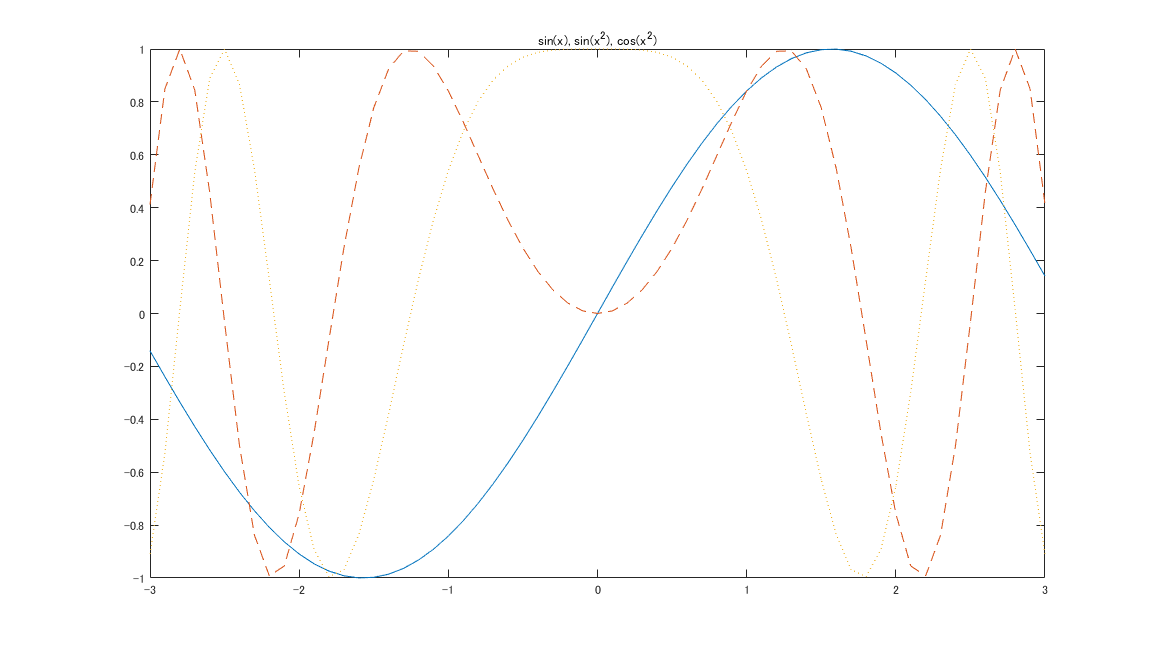
2次元ラインプロット

code

type line2d.m

output

f1=figure(1); clf reset
set(f1,'units','normalized','position',[0.3652 0.3008 0.6016 0.6016])
x=-3:0.1:3;
y1=sin(x);
y2=sin(x.^2);
y3=cos(x.^2);
plot(x,y1,x,y2,'--',x,y3,':')
title('sin(x), sin(x^2), cos(x^2)')

code

line2d

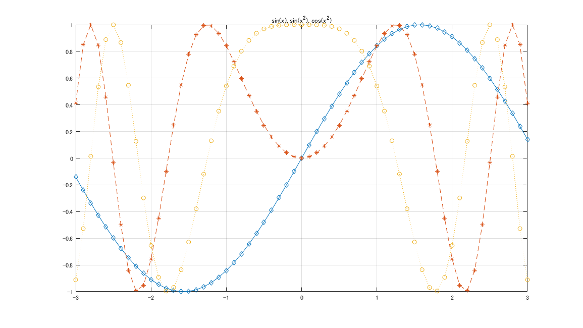
2次元ラインプロット(マーカーつき)

code

h=findobj(gca,'type','line');
set(h(1),'marker','o')
set(h(2),'marker','*')
set(h(3),'marker','d')
grid on

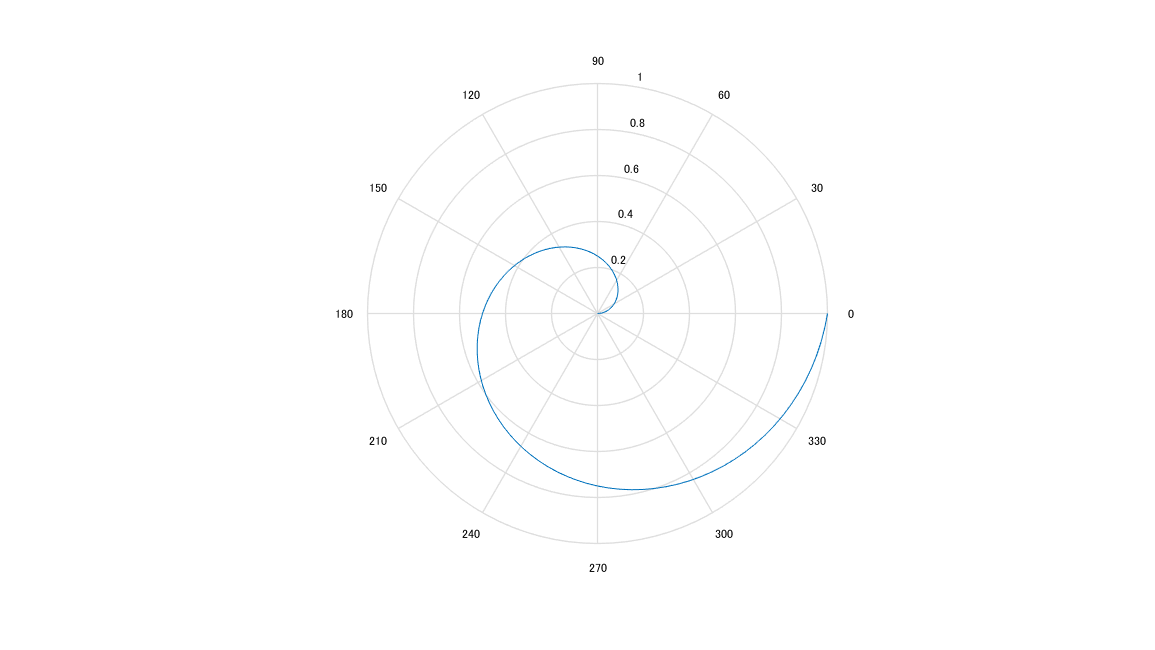
極座標プロット (polar)

code

type polarplot.m

output

f1=figure(1); clf reset
set(f1,'units','normalized','position',[0.3652 0.3008 0.6016 0.6016])

theta=0:2*pi/100:2*pi;
r=theta/(2*pi);
polar(theta,r)

code

polarplot

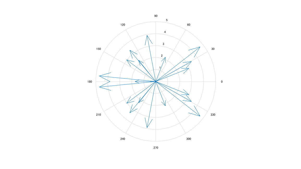
コンパスプロット

code

type compassplot.m

output

f1=figure(1); clf reset
set(f1,'units','normalized','position',[0.3652 0.3008 0.6016 0.6016])

Z = eig(randn(20,20));
compass(Z)

code

compassplot

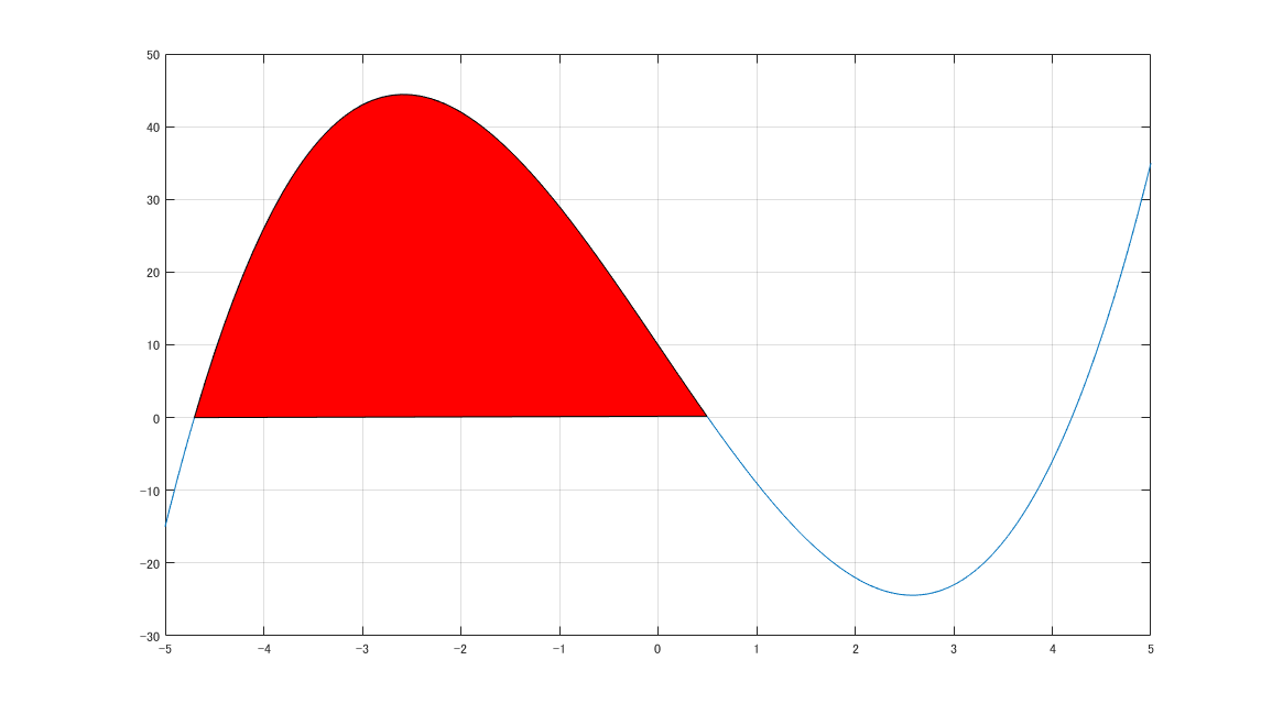
領域の塗りつぶし (fill)

code

type fill2d.m

output

f1=figure(1); clf reset
set(f1,'units','normalized','position',[0.3652 0.3008 0.6016 0.6016])

x=-5:0.05:5;
p=[1 0 -20 10];
y=polyval(p,x);
r=sort(roots(p));
x1=r(1):0.1:r(2);
y1=polyval(p,x1);
plot(x,y)
hold on
fill(x1,y1,'r')
grid

code

fill2d

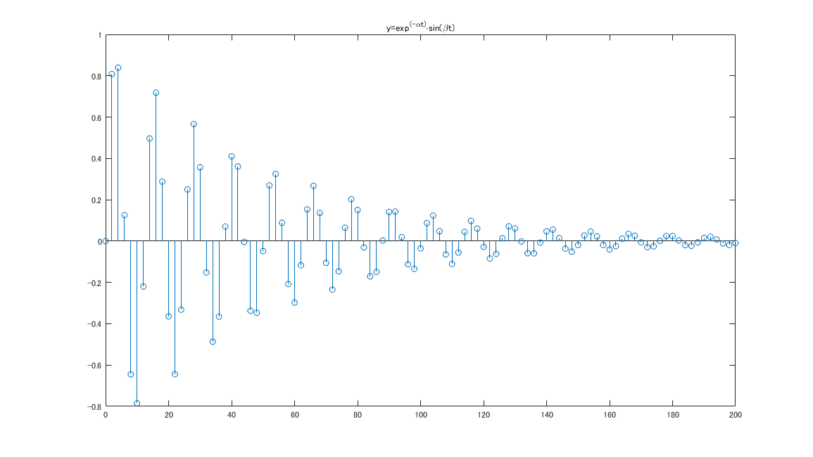
2次元離散プロット (stem)

code

type stem2d.m

output

f1=figure(1); clf reset
set(f1,'units','normalized','position',[0.3652 0.3008 0.6016 0.6016])

alpha=0.02; beta=0.5;
t=0:2:200;
y=exp(-alpha*t).*sin(beta*t);
stem(t,y)
title('y=exp^{(-\alphat)}\cdotsin(\betat)')

code

stem2d

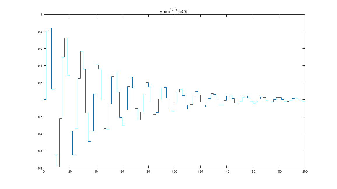
階段状プロット (stairs)

code

type stair2d.m

output

f1=figure(1); clf reset
set(f1,'units','normalized','position',[0.3652 0.3008 0.6016 0.6016])

alpha=0.02; beta=0.5;
t=0:2:200;
y=exp(-alpha*t).*sin(beta*t);
stairs(t,y)
title('y=exp^{(-\alphat)}\cdotsin(\betat)')

code

stair2d

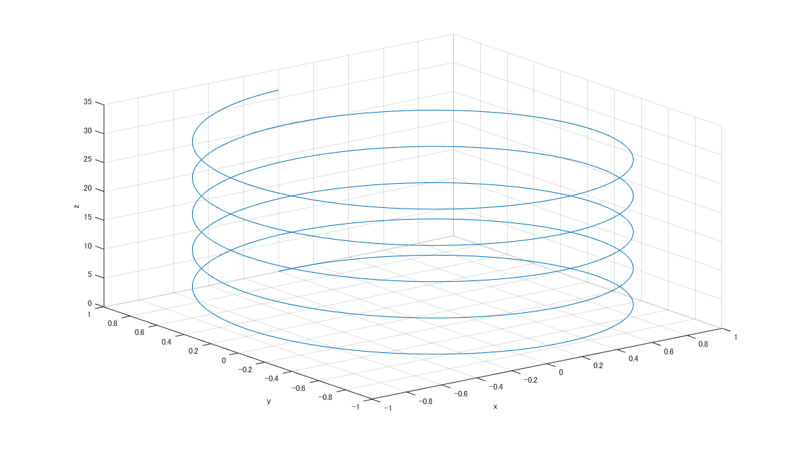
3次元ラインプロット

code

type line3d.m

output

f1=figure(1); clf reset
set(f1,'units','normalized','position',[0.3652 0.3008 0.6016 0.6016])

t=0:pi/50:10*pi;
plot3(sin(t),cos(t),t);
grid
xlabel('x')
ylabel('y')
zlabel('z')

code

line3d

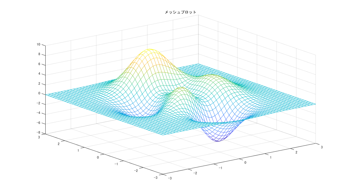
メッシュプロット (mesh)

code

type meshdemo.m

output

f1=figure(1); clf reset
set(f1,'units','normalized','position',[0.3652 0.3008 0.6016 0.6016])

[x,y,z]=peaks(50);
mesh(x,y,z)
title('メッシュプロット','fontname','ＭＳ ゴシック')

code

meshdemo

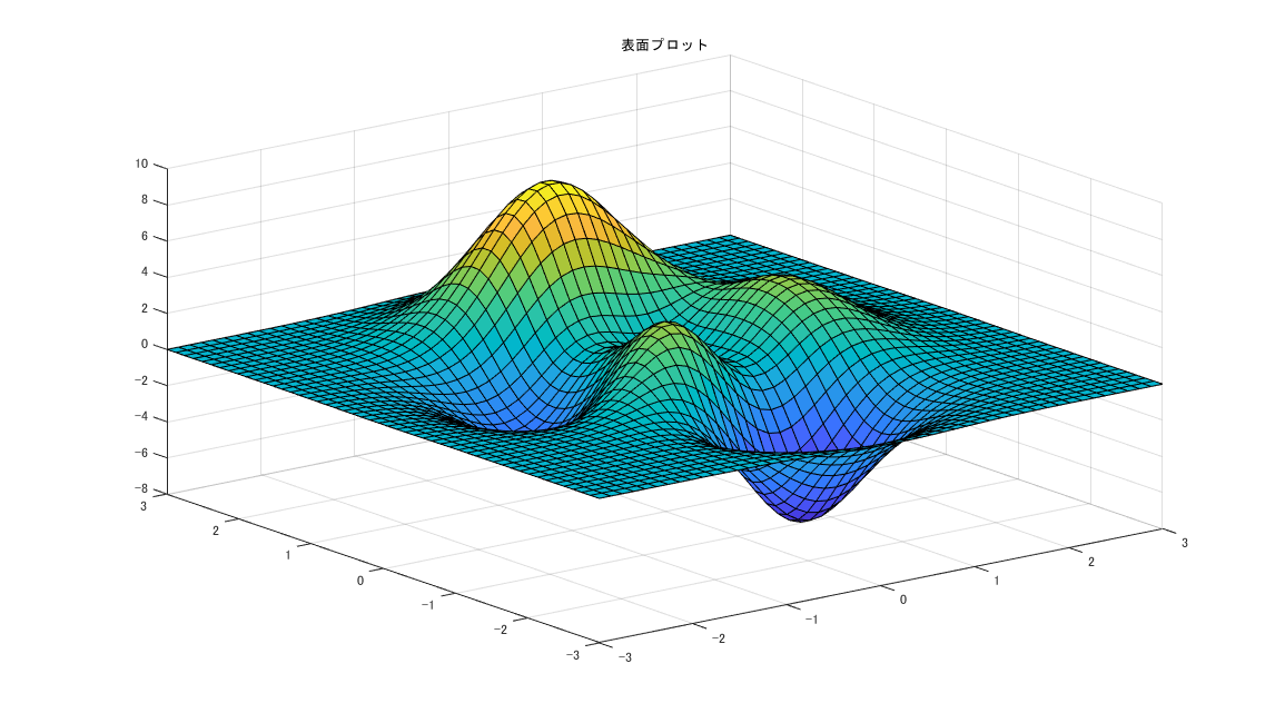
表面プロット (surf)

code

type surfdemo.m

output

f1=figure(1); clf reset
set(f1,'units','normalized','position',[0.3652 0.3008 0.6016 0.6016])

[x,y,z]=peaks(50);
surf(x,y,z)
title('表面プロット','fontname','ＭＳ ゴシック')

code

surfdemo

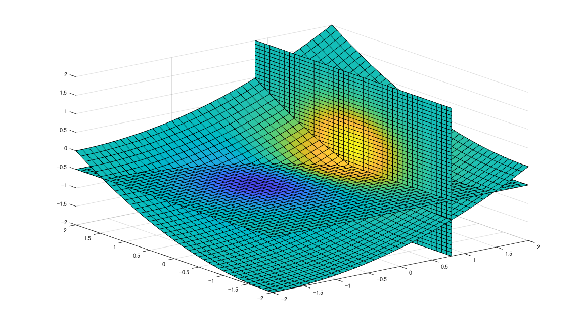
3次元断面プロット (slice)

code

type slicedemo.m

output

f1=figure(1); clf reset
set(f1,'units','normalized','position',[0.3652 0.3008 0.6016 0.6016])

[x,y,z] = meshgrid(-2:.1:2, -2:.1:2, -2:.1:2);
v = x .* exp(-x.^2 - y.^2 - z.^2);

[xi,yi]=meshgrid(0:.1:4);
zi=xi.^2+yi.^2;

slice(x,y,z,v,[.8 ],[],[ -.5])
hold on
slice(x,y,z,v,xi-2,yi-2,zi/8-2);
hold off

code

slicedemo

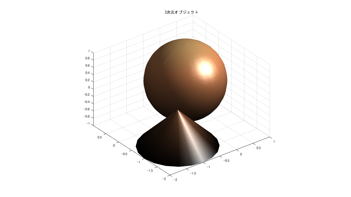
3次元オブジェクト (surf)

code

type obj3d1.m

output

f1=figure(1); clf reset
set(f1,'units','normalized','position',[0.3652 0.3008 0.6016 0.6016])

[x1,y1,z1]=sphere(30);
[x2,y2,z2]=cylinder(1:-0.05:0,20);
x2=x2-1;
y2=y2-1;
z2=z2-1;
surf(x1,y1,z1)
hold on
surf(x2,y2,z2)
light('position',[1 -1 1]);
shading interp
lighting phong
colormap(copper)
axis equal
title('3次元オブジェクト','fontname','ＭＳ ゴシック')

code

obj3d1

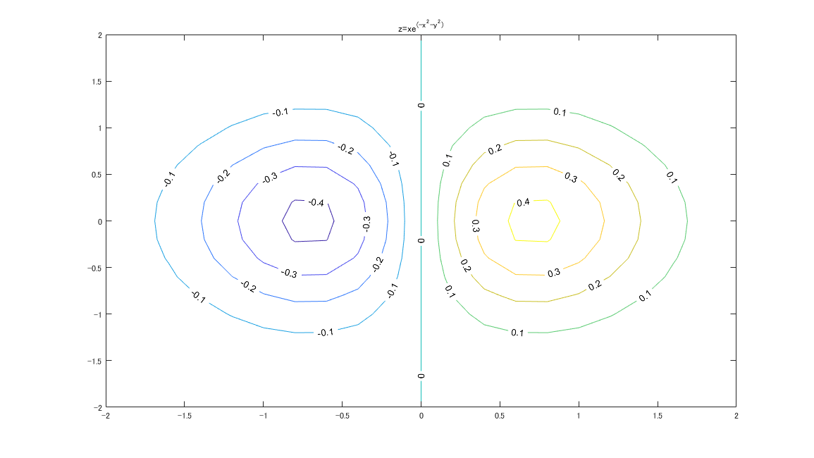
2次元等高線図 (contour)

code

type cont2d.m

output

f1=figure(1); clf reset
set(f1,'units','normalized','position',[0.3652 0.3008 0.6016 0.6016])

[X,Y]=meshgrid(-2:.2:2,-2:.2:2);
Z = X.*exp(-X.^2-Y.^2);
[c,h]=contour(X,Y,Z);
clabel(c,h)
title('z=xe^{(-x^2-y^2)}')

code

cont2d

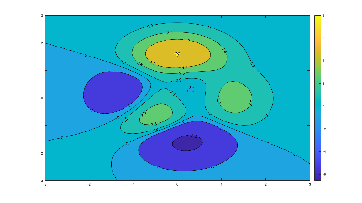
塗りつぶし2次元等高線図

code

type cont2df.m

output

f1=figure(1); clf reset
set(f1,'units','normalized','position',[0.3652 0.3008 0.6016 0.6016])

[X,Y,Z]=peaks;
[c,h]=contourf(X,Y,Z,[-7 -5.5 -1 0 0.9 2.6 4.7 8]);
clabel(c,h)
colorbar

code

cont2df

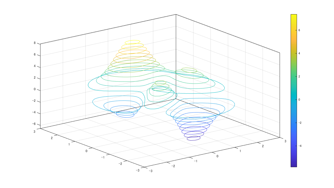
3次元等高線図 (contour3)

code

type cont3d.m

output

f1=figure(1); clf reset
set(f1,'units','normalized','position',[0.3652 0.3008 0.6016 0.6016])

[X,Y,Z]=peaks;
contour3(X,Y,Z,20)
colorbar

code

cont3d

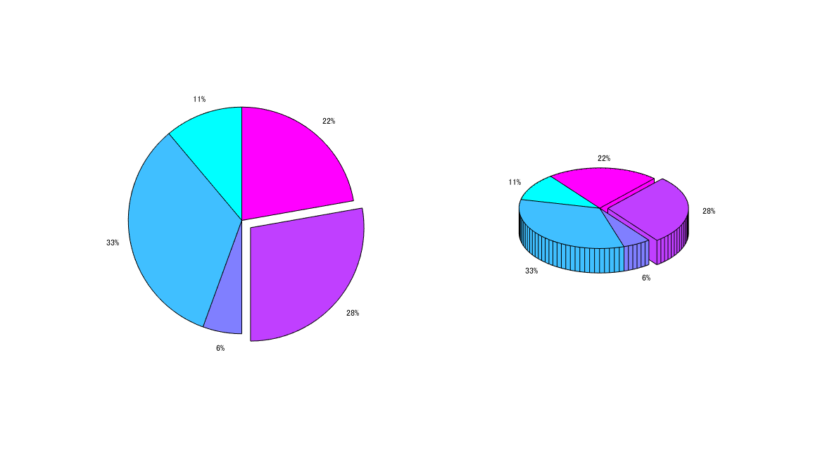
円グラフ (pie)

code

type piedemo.m

output

f1=figure(1); clf reset
set(f1,'units','normalized','position',[0.3652 0.3008 0.6016 0.6016])

x=[1 3 0.5 2.5 2];
explode=[0 0 0 1 0];
subplot(1,2,1),pie(x,explode)
subplot(1,2,2),pie3(x,explode);
colormap(cool)

code

piedemo

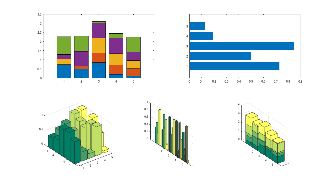
棒グラフ

code

type bargraph.m

output

f1=figure(1); clf reset
set(f1,'units','normalized','position',[0.3652 0.3008 0.6016 0.6016])

Y=rand(5);
subplot(2,2,1),bar(Y,'stacked')
subplot(2,2,2),barh(Y(:,1)) 

X=rand(5);
subplot(2,3,4),bar3(X), set(gca,'ylim',[0 6])
subplot(2,3,5),bar3(X,'grouped')
subplot(2,3,6),bar3(X,'stacked')
colormap(summer)

code

bargraph

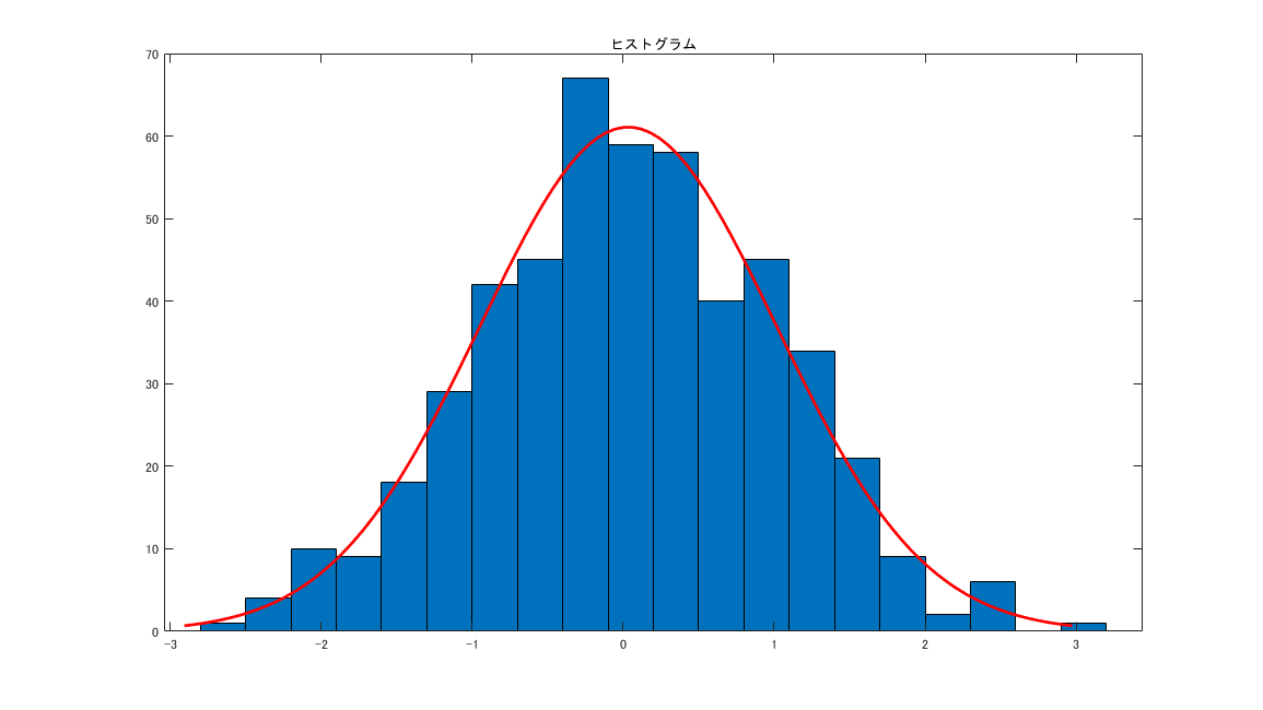
ヒストグラム (hist)

code

type histplot.m

output

f1=figure(1); clf reset
set(f1,'units','normalized','position',[0.3652 0.3008 0.6016 0.6016])

x=randn(500,1);
hist(x,20)
title('ヒストグラム','fontname','ＭＳ ゴシック')

histfit(x,20)
title('ヒストグラム','fontname','ＭＳ ゴシック')

code

histplot

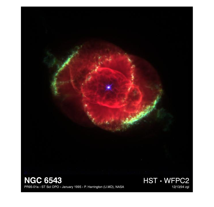
画像表示 (imshow)

code

type implot.m

output

f1=figure(1); clf reset
set(f1,'units','normalized','position',[0.3652 0.3008 0.6016 0.6016])

imshow(imread('ngc6543a.jpg'))

code

implot

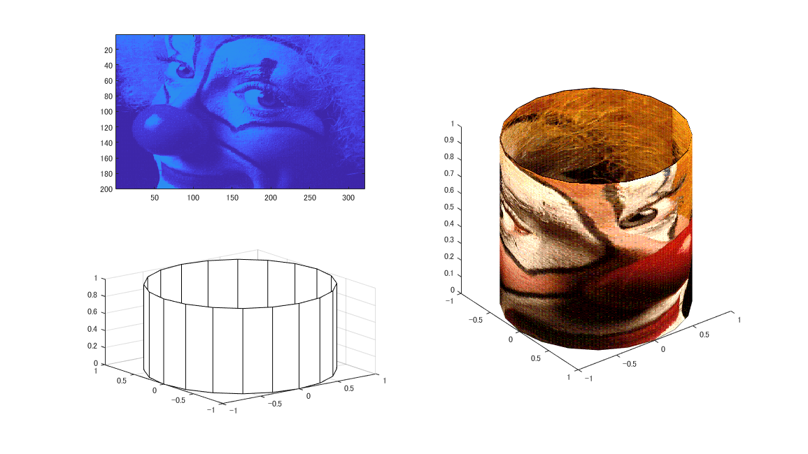
表面プロットへの貼り付け(warp)

code

type warpdemo.m

output

f1=figure(1); clf reset
set(f1,'units','normalized','position',[0.3652 0.3008 0.6016 0.6016])

load clown
[x,y,z]=cylinder;

subplot(2,2,1)
image(X)
axis image

subplot(2,2,3)
h=mesh(x,y,z);
set(h,'edgecolor',[0 0 0])

subplot(122)
warp(x,y,z,flipud(X),map)
axis square

code

warpdemo

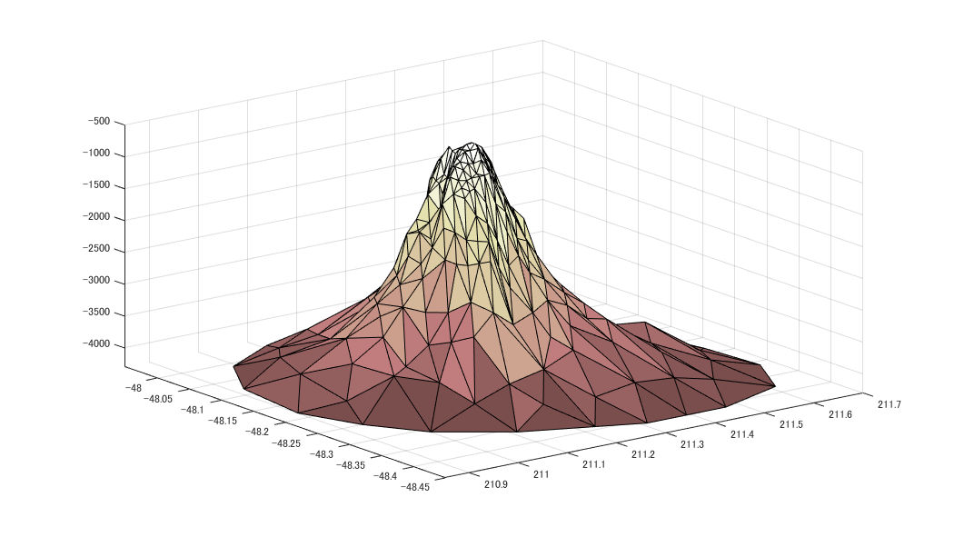
Delaunayの三角メッシュ

code

type tridemo.m

output

f1=figure(1); clf reset
set(f1,'units','normalized','position',[0.0098 0.3529 0.5469 0.5469])
load seamount
tr=delaunay(x,y);
trisurf(tr,x,y,z)
axis([210.85 211.7 -48.45 -47.95 -4300 -500])
map=pink(64);
colormap(map(10:end,:))

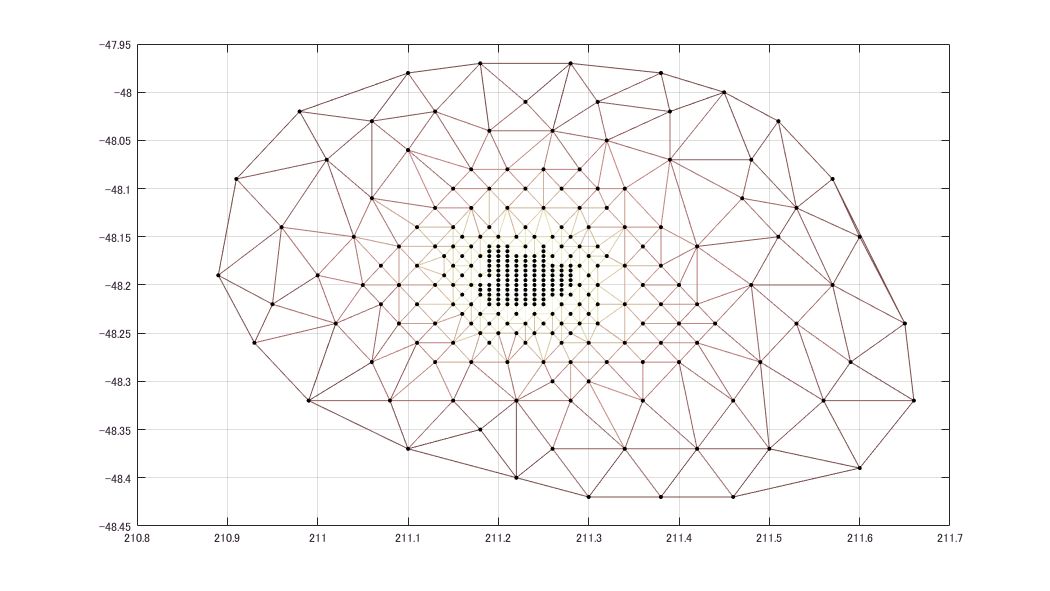
f2=figure(2); clf reset
set(f2,'units','normalized','position',[0.4385 0.0182 0.5469 0.5469])
plot(x,y,'k.','markersize',10)
hold on
trimesh(tr,x,y,z)
hidden off
grid
map=pink(64);
colormap(map(10:end,:))

code

tridemo

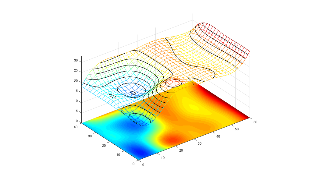
メッシュ、コンター

code

type meshcontour.m

output

f1=figure(1); clf reset
set(f1,'units','normalized','position',[0.0098 0.3529 0.5469 0.5469])
load data3d1
h=surf(x(:,:,30),y(:,:,30),130*ones(21,31)-130,v(:,:,30)*30-125);
%set(h,'edgecolor','none')
shading interp
hold on
h=mesh(x(:,:,30),y(:,:,30),v(:,:,30)*30-125);
set(h,'facecolor','none')
[c,h]=contour3(x(:,:,30),y(:,:,30),v(:,:,30)*30-125,10,'k');
set(h,'linewidth',1)
axis equal
map=jet(64);
colormap(map(10:end,:))

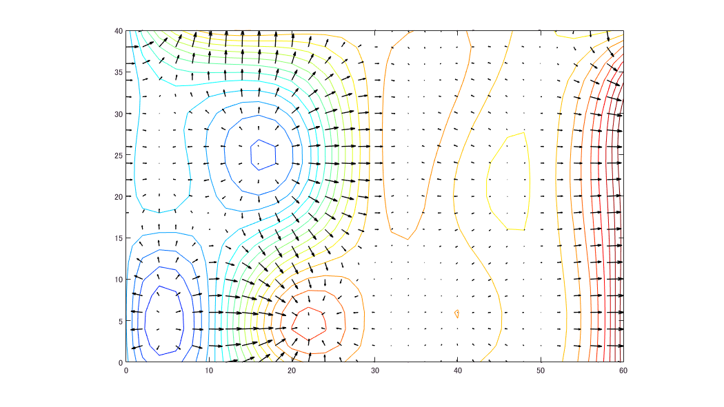
f2=figure(2); clf reset
set(f2,'units','normalized','position',[0.4385 0.0182 0.5469 0.5469])
[px,py]=gradient(v(:,:,30));
contour(x(:,:,30),y(:,:,30),v(:,:,30),20)
hold on
h=quiver(x(:,:,30),y(:,:,30),px,py);
set(h,'color','k','linewidth',1)
axis equal
axis([0 60 0 40])
map=jet(64);
colormap(map(10:end,:))

code

meshcontour

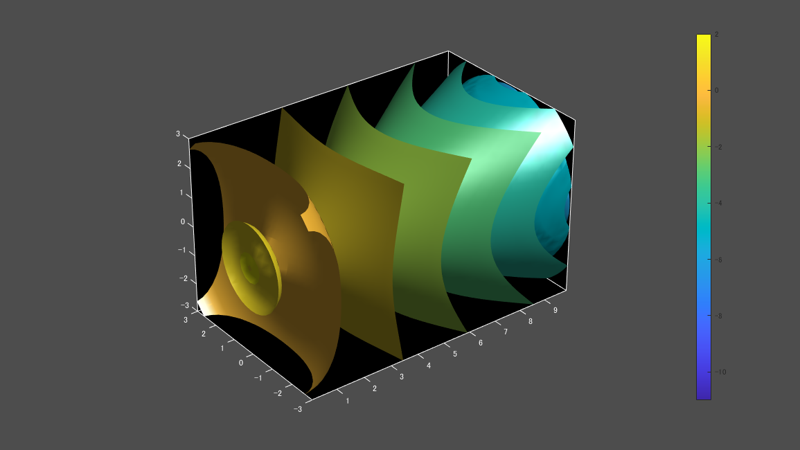
流速の等値面

code

type flowiso2.m

output

f1=figure(1); clf reset
set(f1,'units','normalized','position',[0.3652 0.3008 0.6016 0.6016])

[x y z v] = flow;
p = patch(isosurface(x, y, z, v, 0));
isonormals(x,y,z,v,p);
set(p, 'facecolor', 'r', 'edgecolor', 'n');
daspect([1 1 1]);
view(3);
camlight 
lighting p
%isolims(x,y,z,v)
camproj p; 

delete(p)

for i = -11:2
  p = patch(isosurface(x, y, z, v, i, 'v'));
  isonormals(x,y,z,v,p);
  set(p, 'facec', 'f', 'cdata', i, 'edgec', 'n');
end

set(gcf, 'color', [.3 .3 .3])
set(gca, 'color', 'k')
set(gca, 'xcolor', 'w')
set(gca, 'ycolor', 'w')
set(gca, 'zcolor', 'w')
box on
% lighting g
lighting phong
colorbar;

axis tight

p = findobj('type', 'patch');
caxis(caxis)

code

flowiso2;

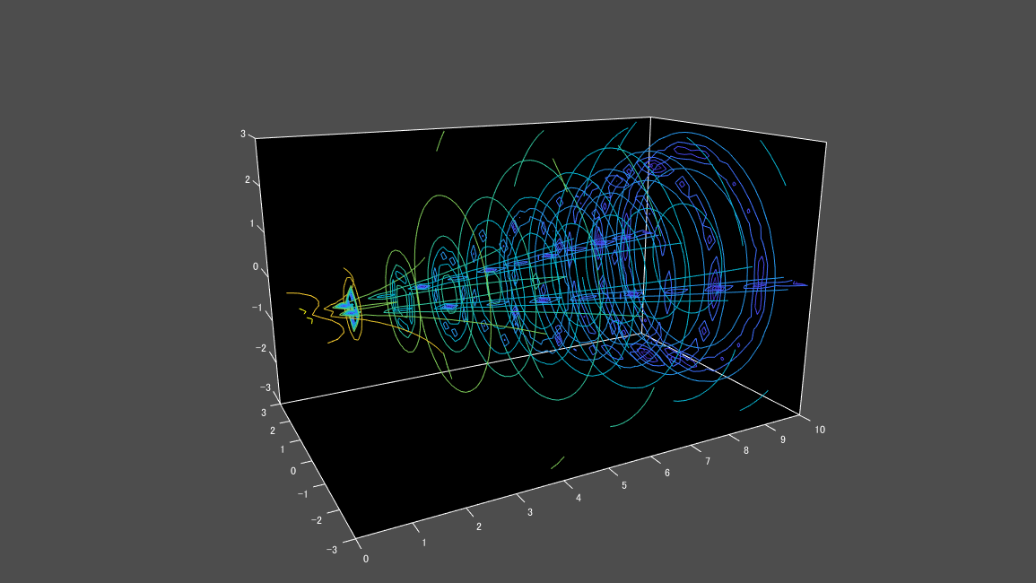
スライス平面上に等高線

code

type cslice.m

output

f1=figure(1); clf reset
set(f1,'units','normalized','position',[0.3652 0.3008 0.6016 0.6016])

[x y z v] = flow;
h=contourslice(x,y,z,v,[1:9],[],[0], linspace(-8,2,10));
axis([0 10 -3 3 -3 3]); daspect([1 1 1])
camva(32); camproj perspective;
campos([-3 -15 5])
set(gcf, 'Color', [.3 .3 .3], 'renderer', 'zbuffer')
set(gca, 'Color', 'black' , 'XColor', 'white', ...
         'YColor', 'white' , 'ZColor', 'white')
box on

code

cslice

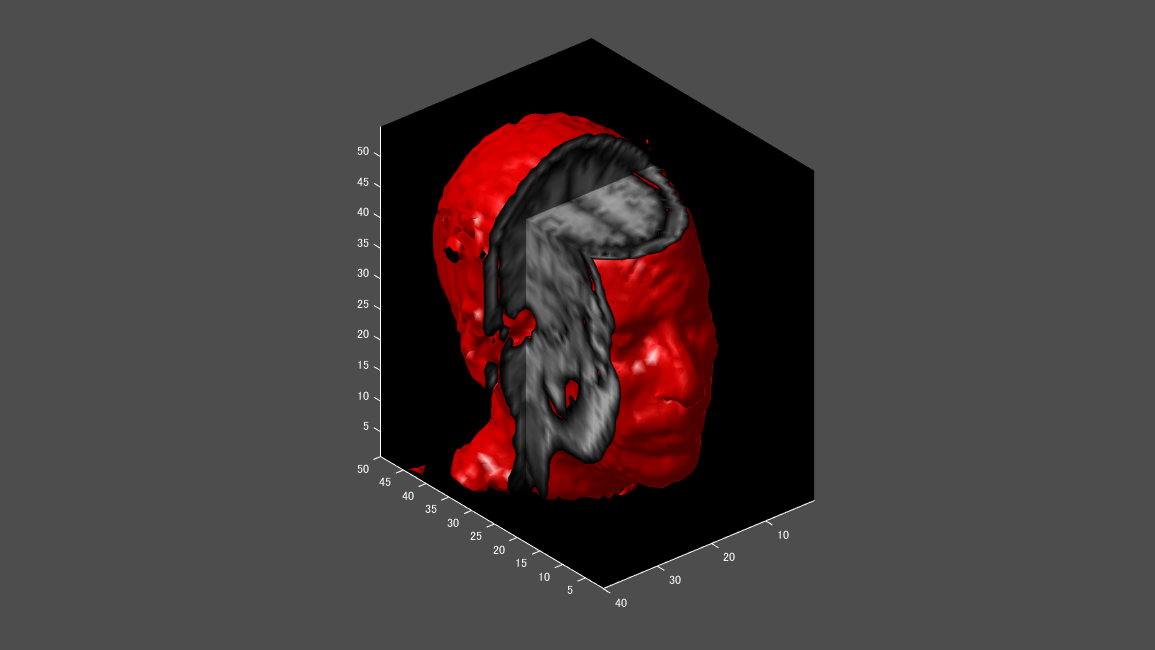
頭部の断面図

code

type headiso_h.m

output

f1=figure(1); clf('reset')
set(f1,'units','normalized','position',[0.3652 0.3008 0.6016 0.6016])

load headsmall
[x y z data2] = subvolume(data, [nan 30    nan 30   nan 45]);
p = patch(isosurface(x,y,z,data2, 30), 'FaceColor', 'r', 'EdgeColor', 'n');
isonormals(x,y,z,data2,p)
p2 = patch(isocaps(x,y,z,data2, 30), 'FaceColor', 'i', 'EdgeColor', 'n');

[x y z data2] = subvolume(data, [30 nan    nan nan   nan nan]);
p = patch(isosurface(x,y,z,data2, 30), 'FaceColor', 'r', 'EdgeColor', 'n');
isonormals(x,y,z,data2, p)
p2 = patch(isocaps(x,y,z,data2, 30), 'FaceColor', 'i', 'EdgeColor', 'n');

view(-130,30);axis vis3d tight; daspect([1 1 1]); h = camlight('left'); 
lighting phong
colormap(gray(100))

set(gcf, 'color', [.3 .3 .3])
set(gca, 'color', 'k')
set(gca, 'xcolor', 'w')
set(gca, 'ycolor', 'w')
set(gca, 'zcolor', 'w')

code

headiso_h

終了

code

% パスを削除
rmpath('.\I1_02_grademo')

参考

MATLAB Plot Gallery

謝辞

本記事は @eigs さんのlivescript2markdownを使わせていただいてます。

目次へのリンク

MATLABによる画像処理・コンピュータービジョン入門目次

1.2 豊富な可視化機能：MATLAB基本関数

目次へのリンク

概要

パスを通す

2次元ラインプロット

2次元ラインプロット(マーカーつき)

極座標プロット (polar)

コンパスプロット

領域の塗りつぶし (fill)

2次元離散プロット (stem)

階段状プロット (stairs)

3次元ラインプロット

メッシュプロット (mesh)

表面プロット (surf)

3次元断面プロット (slice)

3次元オブジェクト (surf)

2次元等高線図 (contour)

塗りつぶし2次元等高線図

3次元等高線図 (contour3)

円グラフ (pie)

棒グラフ

ヒストグラム (hist)

画像表示 (imshow)

表面プロットへの貼り付け(warp)

Delaunayの三角メッシュ

メッシュ、コンター

流速の等値面

スライス平面上に等高線

頭部の断面図

終了

参考

謝辞

目次へのリンク