こんにちは
今回は Pythonで作成した分析モデルをVantageで活用する方法について解説したいと思います。
使いなれたPythonで分析モデルを作成頂き Vantageにインポートして頂く事で Vantage内にあるデータを高速にスコアリングする事が可能です。

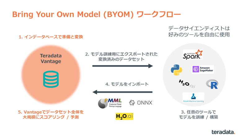
この記事はTeradata VantageとTeradatamlを使用してPyhtonで作成した分析モデルをBYOM(Bring Your Own Meeting)してVantageにインポートする事で業務に活用する流れを説明します。
Vantage の BYOM は現在 PMML, ONNX, H2O MOJO フォーマットに対応しています。

はじめに

使用するデータは scikit-learnの機械学習でロジスティック回帰を行い癌の陽性を判断するためのサンプルデータ(load_breast_cancer) を利用します。
あらかじめ Vantageに load_breast_cancer と言うテーブルを作成しサンプルデータを格納しておきます。

入力テーブル(load_breast_cancer)

データ件数 : 569件
説明変数 : 30個
目的変数 : 1個(0:陰性/1:陽性)
その他 :
uidと言う連番カラムを追加しています。
説明変数と目的変数は結合し目的変数としてtargetカラムを追加しています。

uid	mean_radius	mean_texture	mean_perimeter	mean_area	mean_smoothness	mean_compactness	mean_concavity	mean_concave_points	mean_symmetry	mean_fractal_dimension	radius_error	texture_error	perimeter_error	area_error	smoothness_error	compactness_error	concavity_error	concave_points_error	symmetry_error	fractal_dimension_error	worst_radius	worst_texture	worst_perimeter	worst_area	worst_smoothness	worst_compactness	worst_concavity	worst_concave_points	worst_symmetry	worst_fractal_dimension	target
1	6.981	13.43	43.79	143.5	0.117	0.07568	0.0	0.0	0.193	0.07818	0.2241	1.508	1.553	9.833	0.01019	0.01084	0.0	0.0	0.02659	0.0041	7.93	19.54	50.41	185.2	0.1584	0.1202	0.0	0.0	0.2932	0.09382	1
2	7.691	25.44	48.34	170.4	0.08668	0.1199	0.09252	0.01364	0.2037	0.07751	0.2196	1.479	1.445	11.73	0.01547	0.06457	0.09252	0.01364	0.02105	0.007551	8.678	31.89	54.49	223.6	0.1596	0.3064	0.3393	0.05	0.279	0.1066	1
3	7.729	25.49	47.98	178.8	0.08098	0.04878	0.0	0.0	0.187	0.07285	0.3777	1.462	2.492	19.14	0.01266	0.009692	0.0	0.0	0.02882	0.006872	9.077	30.92	57.17	248.0	0.1256	0.0834	0.0	0.0	0.3058	0.09938	1
4	7.76	24.54	47.92	181.0	0.05263	0.04362	0.0	0.0	0.1587	0.05884	0.3857	1.428	2.548	19.15	0.007189	0.00466	0.0	0.0	0.02676	0.002783	9.456	30.37	59.16	268.6	0.08996	0.06444	0.0	0.0	0.2871	0.07039	1
5	8.196	16.84	51.71	201.9	0.086	0.05943	0.01588	0.005917	0.1769	0.06503	0.1563	0.9567	1.094	8.205	0.008968	0.01646	0.01588	0.005917	0.02574	0.002582	8.964	21.96	57.26	242.2	0.1297	0.1357	0.0688	0.02564	0.3105	0.07409	1

(サンプル5件)

1. 環境の準備

a. データベース環境の準備

PMMLをデータベースで作成するための権限(EXECUTE FUNCTION権限)を実行ユーザに付与します。

sql

GRANT EXECUTE FUNCTION ON mldb TO {実行ユーザ};

b. #Python環境の準備(初回必要な作業です)

pip install teradataml --upgrade
pip install sklearn
pip install sklearn2pmml
pip install jdk4py --user

jdk4py は javaのランタイムです。
PMMLファイル作成に Javaのランタイムが必要です。
環境変数にjavaランタイムのPATHを追加する必要があります。

ex.

PATH=$PATH:/home/jovyan/.local/lib/python3.9/site-packages/jdk4py/java-runtime/bin

2. サンプルデータを準備する

python

# 基本的なライブラリの読み込み
import pandas as pd
from teradataml.context.context import *
from teradataml import DataFrame,copy_to_sql

# データベースに接続
create_context(host='192.168.1.232',username='sysdba',password='sysdba')

# 癌のデータをDataFrameにロードする
source_df=DataFrame("load_breast_cancer")

# 説明変数のカラムリストを用意
features=[ "mean_radius"
,"mean_texture"
,"mean_perimeter"
,"mean_area"
,"mean_smoothness"
,"mean_compactness"
,"mean_concavity"
,"mean_concave_points"
,"mean_symmetry"
,"mean_fractal_dimension"
,"radius_error"
,"texture_error"
,"perimeter_error"
,"area_error"
,"smoothness_error"
,"compactness_error"
,"concavity_error"
,"concave_points_error"
,"symmetry_error"
,"fractal_dimension_error"
,"worst_radius"
,"worst_texture"
,"worst_perimeter"
,"worst_area"
,"worst_smoothness"
,"worst_compactness"
,"worst_concavity"
,"worst_concave_points"
,"worst_symmetry"
,"worst_fractal_dimension"]

# 目的変数のカラムリストを用意
target=['target']

3. サンプルデータを訓練用と評価用に分割する

python

from sklearn.model_selection import train_test_split

#データの分割を行う（訓練用データ 0.8 評価用データ 0.2）
dataX = source_df.select(features).to_pandas()
dataY = source_df.select(target).to_pandas()
X_train, X_test, y_train, y_test = train_test_split(dataX, dataY, test_size=0.2)

4. 訓練用データでモデルを作成する

python

from sklearn import linear_model
from sklearn2pmml.pipeline import PMMLPipeline

#線形モデル(ロジスティク回帰)として測定器を作成する
clf = linear_model.LogisticRegression(max_iter=20000)

# Create a pipeline consisting of a single step: the classifier
rf_pipeline = PMMLPipeline([
    ("liner",clf)
])

#訓練の実施
rf_pipeline.fit(X_train,y_train)

5. モデルを評価する

a. 行ごとに陰性と陽性の確立を表示

python

#評価の実行（確率）
df = pd.DataFrame(rf_pipeline.predict_proba(X_test))
df = df.rename(columns={0: '確率(陰性)',1: '確率(陽性)'})
df.head(5)

結果を5行表示します

	確率(陰性)	確率(陽性)
0	1.000000	1.329340e-10
1	0.955834	4.416590e-02
2	0.988545	1.145463e-02
3	0.999999	9.603573e-07
4	0.000103	9.998968e-01

・1列目は行番号
・確率(陰性) : 0である確率
・確率(陽性) : 1である確率

b. 行ごとに陰性か陽性の判断

python

#評価の実行（判定）
df = pd.DataFrame(rf_pipeline.predict(X_test))
df = df.rename(columns={0: '判定(0:陰性 / 1:陽性)'})
df.head(5)

結果を5行表示します

	判定(0:陰性 / 1:陽性)
0	0
1	0
2	0
3	0
4	1

・1列目は行番号
・確立から1か0を判定します
　　・確率(陰性) : 0
　　・確率(陽性) : 1

c. 混合行列を表示

python

#混同行列
df = pd.DataFrame(confusion_matrix(y_test,rf_pipeline.predict(X_test).reshape(-1,1), labels=[0,1]))
df = df.rename(columns={0: '予想(0:陰性)',1: '予想(1:陽性)'}, index={0: '実際(0:陰性)',1: '実際(1:陽性)'})
df

結果を表示します

	予想(0:陽性)	予想(1:陽性)
実際(0:陽性)	40	6
実際(1:陽性)	2	66

縦は予測を表し横は実際を表します
表内の数字は
　・0と予測して実際は0であった比率。
　・0と予測して実際は1であった比率。
　・1と予測して実際は0であった比率。
　・1と予測して実際は1であった比率。

d. 正答率を表示

python

#評価の実行（正答率）
rf_pipeline.score(X_test,y_test)

全体の正答率を表示します

0.9298245614035088

分析モデルの精度を確認しパラメータを変更するなどして制度を高めます。
分析モデルが完成したら本題であるBYOMの手順へ進みます。

6. モデルをPMMLに変換してファイルに出力する

python

# # JavaランタイムがPathに設定されていない場合はコメントを解除して追加
# # (ここから)
# import os
# import getpass
# # Javaの環境変数をPathにセット
# os.environ['PATH'] = os.environ['PATH'] + ':/home/jovyan/.local/lib/python3.9/site-packages/jdk4py/java-runtime/bin'
# # (ここまで)

from sklearn2pmml import sklearn2pmml

# PMMLファイルを出力
sklearn2pmml(rf_pipeline, "deomomodel.pmml")

7. モデルをTeradataにインポートする

python

from teradataml import save_byom,delete_byom

# PMMLファイルを Vantageにインポート
model_id   = 'liner'
model_file = 'deomomodel.pmml'
table_name = 'demo_models'

# Try to save the model and overwrite if exists
try:
    # Saving model in PMML format to Vantage table
    res = save_byom(model_id = model_id, model_file = model_file, table_name = table_name)

except Exception as e:
    # if our model exists, delete and rewrite
    if str(e.args).find('TDML_2200') >= 1:
        res = delete_byom(model_id = model_id, table_name = table_name)
        res = save_byom(model_id = model_id, model_file = model_file, table_name = table_name)
        pass
    else:
        raise

8. モデルを使ってTeradataでスコアリング実行

a. Pythonでteradataml関数を使って出力する

python

from teradataml import PMMLPredict

# モデルをデータフレームにセットする
model_tdf = DataFrame.from_query(f"SELECT * FROM {table_name} WHERE model_id = '{model_id}'")

# Vantageのテーブルをスコアリング
configure.byom_install_location = 'mldb'
# Run the PMMLPredict function in Vantage
result = PMMLPredict(
            modeldata = model_tdf.select(['model_id','model']),
            newdata   = source_df,
            accumulate = ['uid'],
            )
result

b. SQL関数を使って出力する

sql

SELECT * FROM mldb.PMMLPredict(
ON load_breast_cancer as InputTable
ON demo_models        as ModelTable DIMENSION 
USING
Accumulate ( 'uid' )
) as T;

・ load_breast_cancer : モデルテーブル
・ demo_models : スコアリング対象テーブル

スコアリング結果のサンプル10件

uid	prediction	json_report
122		{"probability(1)":0.9997953797438303,"probability(0)":2.0462025616974078E-4}
448		{"probability(1)":0.30907169671134693,"probability(0)":0.6909283032886531}
244		{"probability(1)":0.9863827894228404,"probability(0)":0.013617210577159589}
469		{"probability(1)":7.630531300746095E-8,"probability(0)":0.999999923694687}
326		{"probability(1)":0.9329955969490824,"probability(0)":0.0670044030509176}
183		{"probability(1)":0.9999383527073827,"probability(0)":6.164729261726176E-5}
40		{"probability(1)":0.9999292699626635,"probability(0)":7.073003733648608E-5}
509		{"probability(1)":0.001220742207517614,"probability(0)":0.9987792577924823}
61		{"probability(1)":0.9999895954415977,"probability(0)":1.0404558402288266E-5}
387		{"probability(1)":0.02058008631907677,"probability(0)":0.9794199136809232}

uid :
Accumulateで指定したカラム名。
prediction :
分類モデルで行われたスコアリングが予測値を返さない場合予測値出力カラムは空になる可能性があります。
回帰モデルや単一のフィールドを返すモデルでスコアリングが行われた場合予測値カラムには値が含まれます。
json_report :
スコアリング結果はJson形式で出力されます。
・probability(0) : 陰性
・probability(1) : 陽性

終わりに

いかがだったでしょうか。
今回は Teradata VantageとTeradatamlを使用してPyhtonで作成した分析モデルをBYOM(Bring Your Own Meeting)してVantageにインポートする事で業務に活用する流れを説明しました。
VantageはPythonに限らず外部で作成した分析モデルをデータベース内にインポートして大規模なテーブルのスコアリングを高速に実行可能です。

警告
この本書はTeradata Vantageドキュメンテーションよりトピックに必要な情報を抜粋したものです。掲載内容の正確性・完全性・信頼性・最新性を保証するものではございません。正確な内容については、原本をご参照下さい。
また、修正が必要な箇所や、ご要望についてはコメントをよろしくお願いします。

Teradata Vantageへのお問合せ

Teradata Vantage へのお問合せ

Pythonの分析モデルをBYOMしてVantageで利用する

はじめに

入力テーブル(load_breast_cancer)

1. 環境の準備

a. データベース環境の準備

b. #Python環境の準備(初回必要な作業です)

2. サンプルデータを準備する

3. サンプルデータを訓練用と評価用に分割する

4. 訓練用データでモデルを作成する

5. モデルを評価する

a. 行ごとに陰性と陽性の確立を表示

b. 行ごとに陰性か陽性の判断

c. 混合行列を表示

d. 正答率を表示

6. モデルをPMMLに変換してファイルに出力する

7. モデルをTeradataにインポートする

8. モデルを使ってTeradataでスコアリング実行

a. Pythonでteradataml関数を使って出力する

b. SQL関数を使って出力する

終わりに

Teradata Vantageへのお問合せ